Background
Sergei Mikhailovich Prokudin-Gorskii (1863-1944) [Сергей Михайлович Прокудин-Горский, to his Russian friends] was a man well ahead of his time. Convinced, as early as 1907, that color photography was the wave of the future,
he won Tzar's special permission to travel across the vast Russian Empire and take color photographs of everything he saw including the only color portrait of Leo Tolstoy. And he really photographed everything: people, buildings,
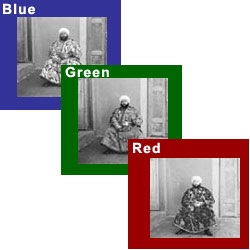
landscapes, railroads, bridges... thousands of color pictures! His idea was simple: record three exposures of every scene onto a glass plate using a red, a green, and a blue filter. Never mind that there was no way to print color
photographs until much later -- he envisioned special projectors to be installed in "multimedia" classrooms all across Russia where the children would be able to learn about their vast country. Alas, his plans never materialized:
he left Russia in 1918, right after the revolution, never to return again. Luckily, his RGB glass plate negatives, capturing the last years of the Russian Empire, survived and were purchased in 1948 by the Library of Congress. The
LoC has recently digitized the negatives and made them available on-line.
Overview
The goal of this assignment is to take the digitized Prokudin-Gorskii glass plate images and, using image processing techniques, automatically produce a color image with as few visual artifacts as possible. In order to do this,
you will need to extract the three color channel images, place them on top of each other, and align them so that they form a single RGB color image. The program will take a glass plate image as input and produce a single color
image as output. The program will then divide the image into three equal parts and align the second and the third parts (e.x. G and R) to the first (B). For each image, you will need to print the (x,y) displacement vector that was
used to align the parts.
Section I: Single-Scale Alignment
We started off working with JPEG images, and since these are compressed, are often at relatively low resolutions. The easiest way to align the parts is to exhaustively search over a window of possible displacements
(say [-15,15] pixels), score each one using some image matching metric, and take the displacement with the best score. There is a number of possible metrics that one could use to score how well the images match. The simplest
one is just the L2 norm also known as the Euclidean Distance which is simply sqrt(sum(sum((image1-image2)^2))) where the sum is taken over the pixel values. Another is Normalized Cross-Correlation (NCC), which is simply a dot
product between two normalized vectors: (image1 / ||image1|| and image2 / ||image2||).
Since these JPEG images are small enough, we can perform this exhaustive single scale search at a relatively low cost. I tried the implementations of 3 different alignment scoring methods: L2 Norm, Normalized Cross-Correlation (NCC), and
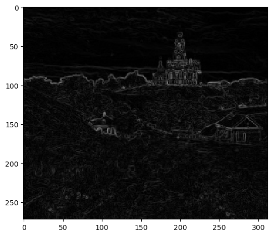
structural similarity (SSIM) and found that NCC and SSIM seemed to get similar results but were better than L2 Norm. In each alignment metric scoring step, we will apply to Sobel filter on the images before scoring to help with
edge detection instead of only having pixel intensity. After getting all 3 color channels aligned, we will merge the channels using np.dstack like so: np.dstack([aligned_red_channel, aligned_green_channel, blue_channel]). Before working
with any image, we will crop 20% all of margins (top, bottom, left, right) from every image to remove any black bars which may skew the alignment scoring.
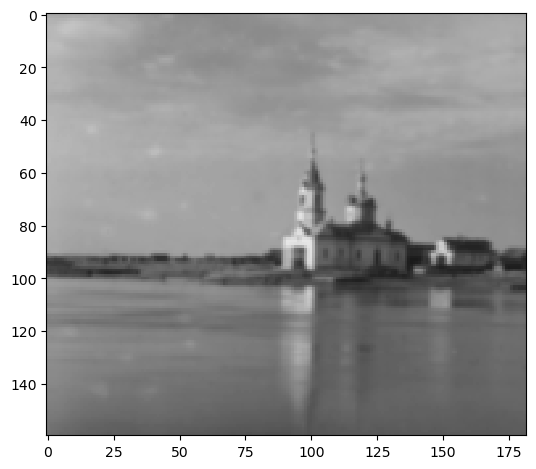
 Sobel Edge Map
|
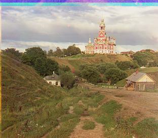
 cathedral.jpg: G(5, 2), R(12, 3)
|
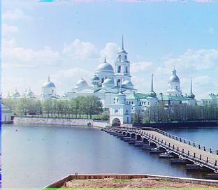
 monastery.jpg: G(-3, 2), R(3, 2)
|
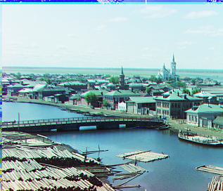
 tobolsk.jpg: G(3, 3), R(6, 3)
|
Section II: Multi-Scale Alignment
Next, we will start working with TIF images, which are much higher quality than JPEG but that also means are often of much higher resolution. This means that our previous single-scale solution will be too expensive to be able to
efficiently align the color channels. This is where we can introduce a coarse-to-fine image pyramid optimization. Here is the breakdown:
We will create a list that will store the original image at varying levels of resolution, with the original resolution being at the bottom (index 0 in this case).
1: First, specify how many levels or how many times we want to scale our resolution down. More means a "taller" pyramid with increasingly lower resolution images.
2: At each level, blur the image and then downscale the image to half of its current size/resolution.
3: Append this image to our list, which is the data structure respresenting our image pyramid.
4: Repeat for however many levels you have specified your pyramid to be.
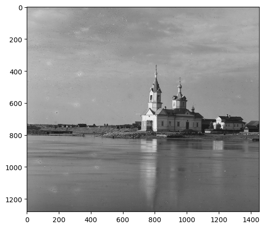
 Pyramid Level 0 (highest resolution)
|
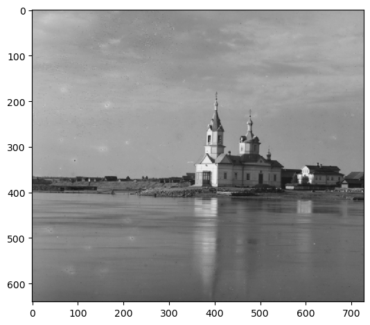
 Pyramid Level 1
|
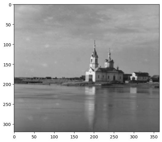
 Pyramid Level 2
|
 Pyramid Level 3
|
 Pyramid Level 4
|
 Pyramid Level 5 (lowest resolution)
|
Now that we have our image pyramid constructed, we can begin our image alignment algorithm. First, we will start at the top level of the pyramid, or the lowest resolution image. Since this image wll be very small, we can have a
larger search space and still be cost-efficient. At this lower level, we will run our previous single-scale alignment algorithm (NCC/SSIM), that will give an initial best displacement vector. Now that we have this displacement vector as a baseline, we
then go down a level in the pyramid to next next higher resolution image. In this step, we will shrink the search space and run the single-scale alignment algorithm again but now we will center this smaller search space around our
baseline best displacement vector (displacement_vector + smaller_search_space). This will then give a newly adjust best displacement vector which we will use in the next step. Since we are going up in resolution after each step,
we will also multiply the "best" displacement vector by 2 each step to account for the doubling in resolution. Essentially, we will iterate through our image pyramid from lowest to highest resolution image, perform a
single-scale alignment step at each iteration but also continuously update our best displacement vector using the previous steps. We shrink the search space at each step so that as the images become higher resolution, the search space
does not become too expensive when aligning. At the last step, we will get a final displacement vector which we can then use to translate the original image.
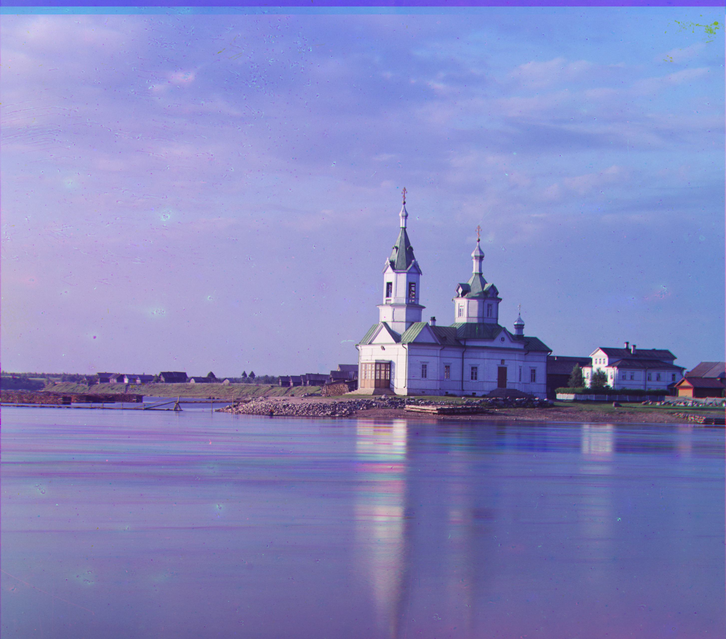
 church.jpg: G(26, 4), R(58, -4)
|
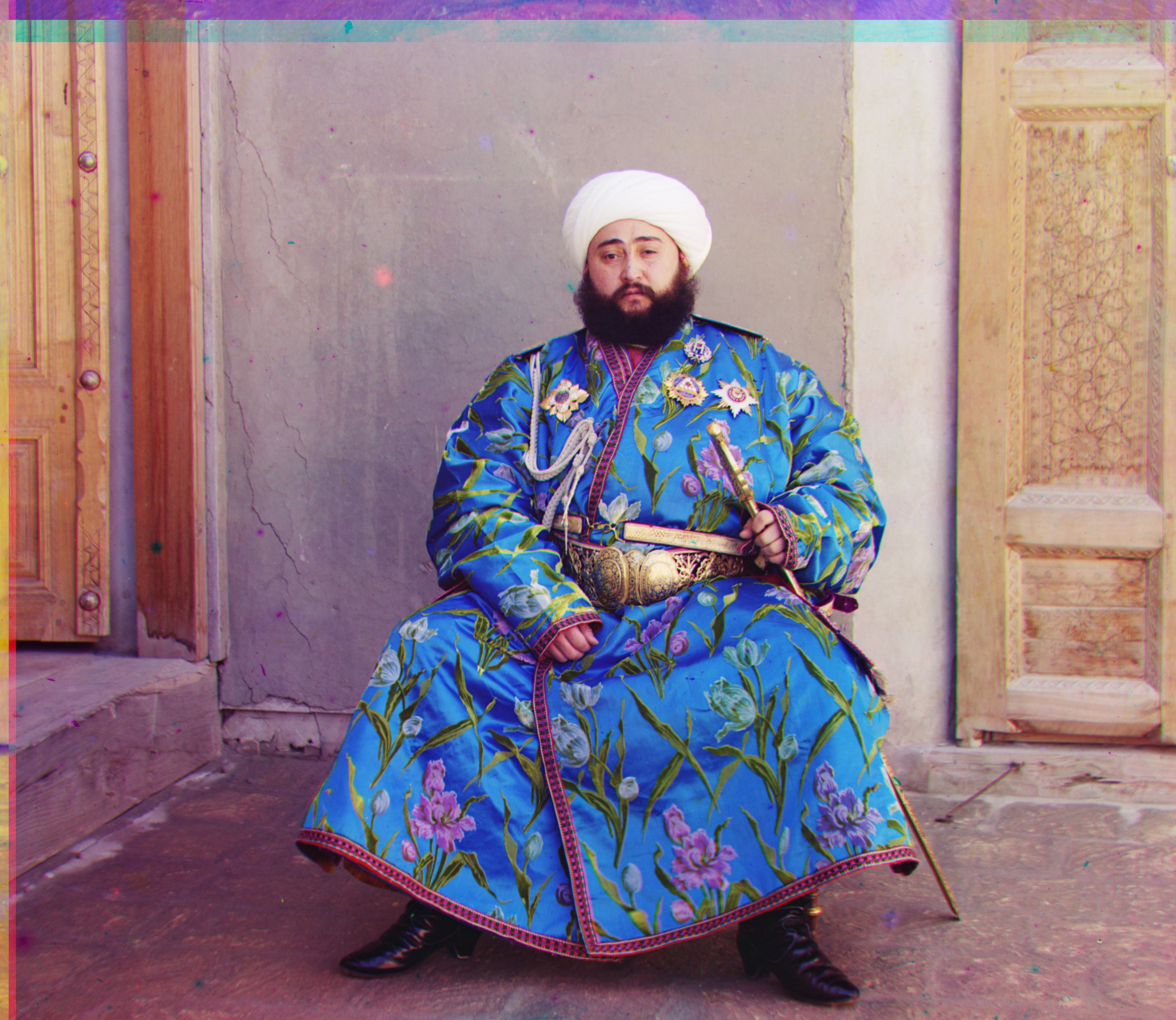
 emir.jpg: G(50, 22), R(106, 40)
|
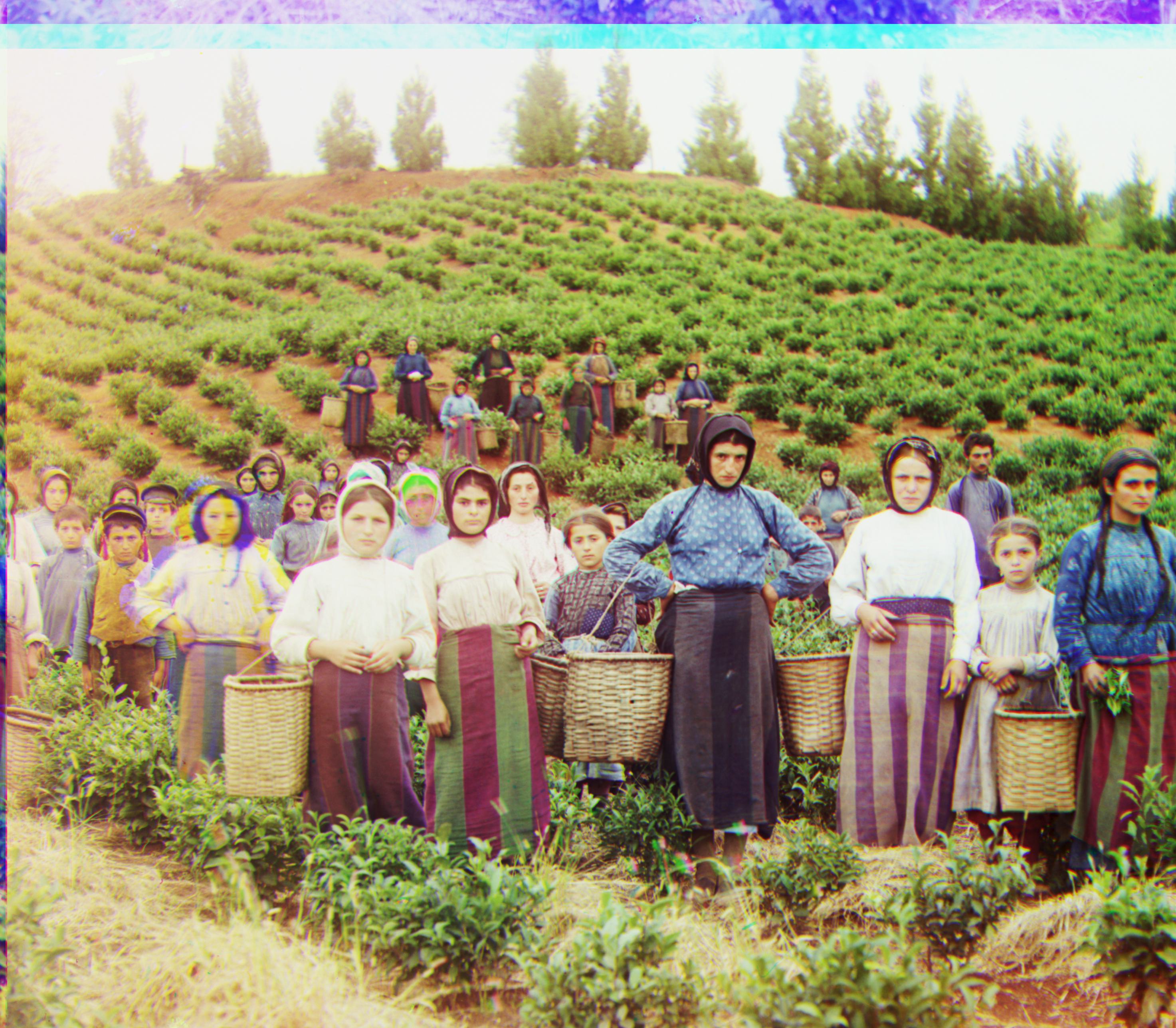
 harvesters.jpg: G(60, 18), R(122, 14)
|
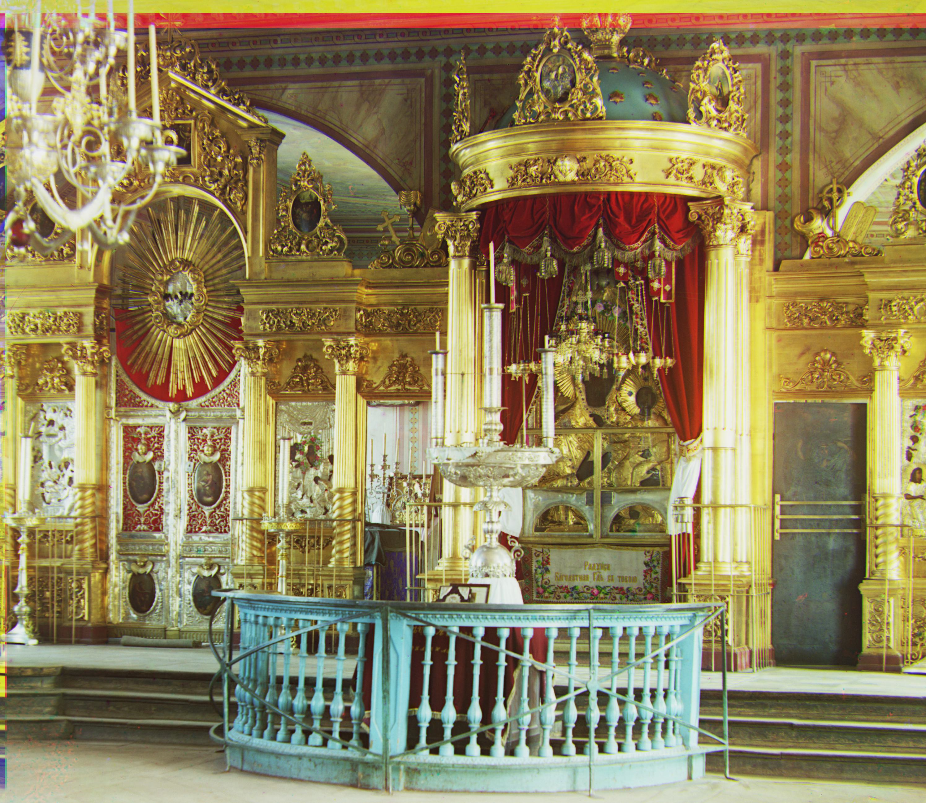 icon.jpg: G(42, 16), R(90, 22)
|
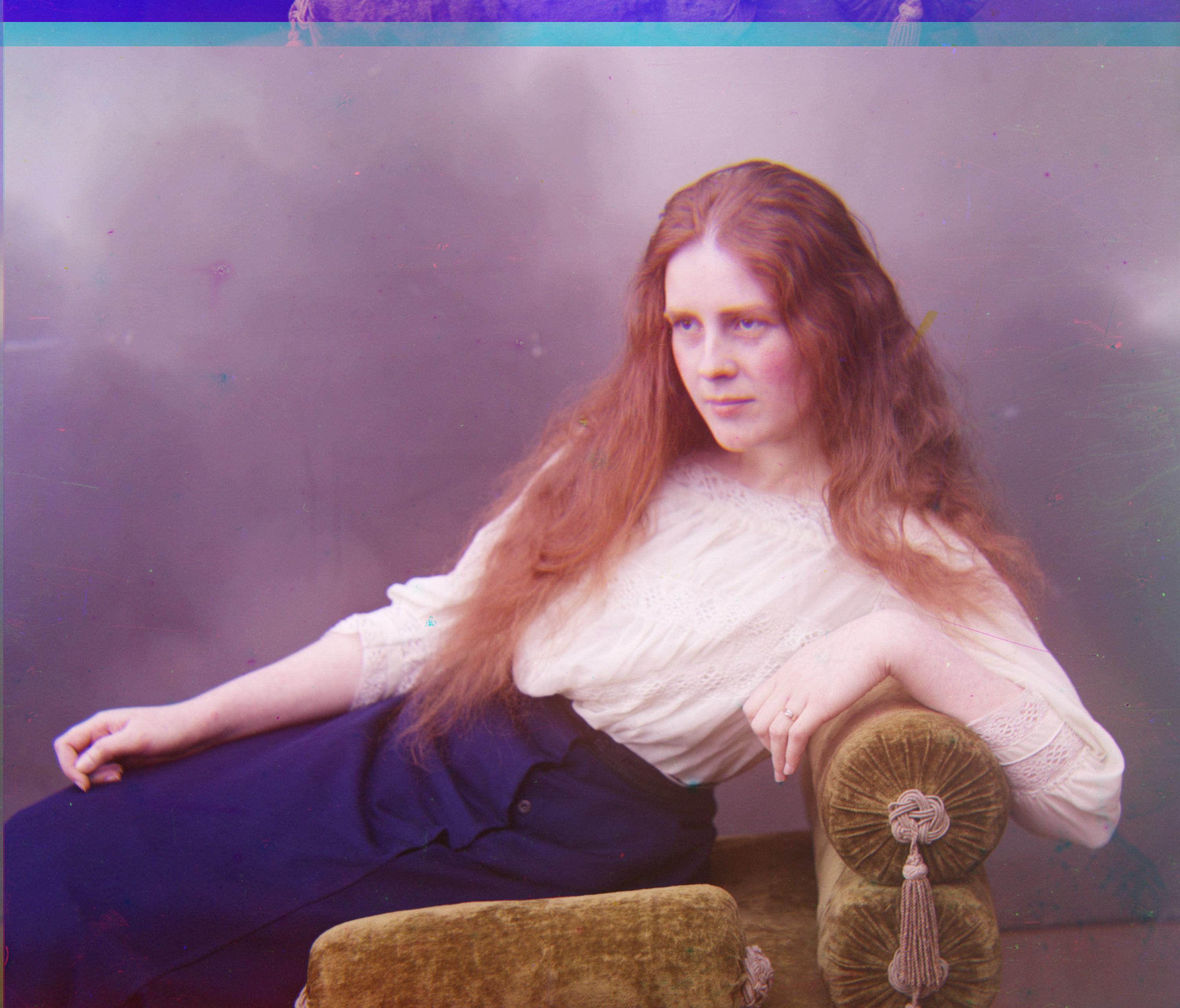
 lady.jpg: G(56, 8), R(118, 12)
|
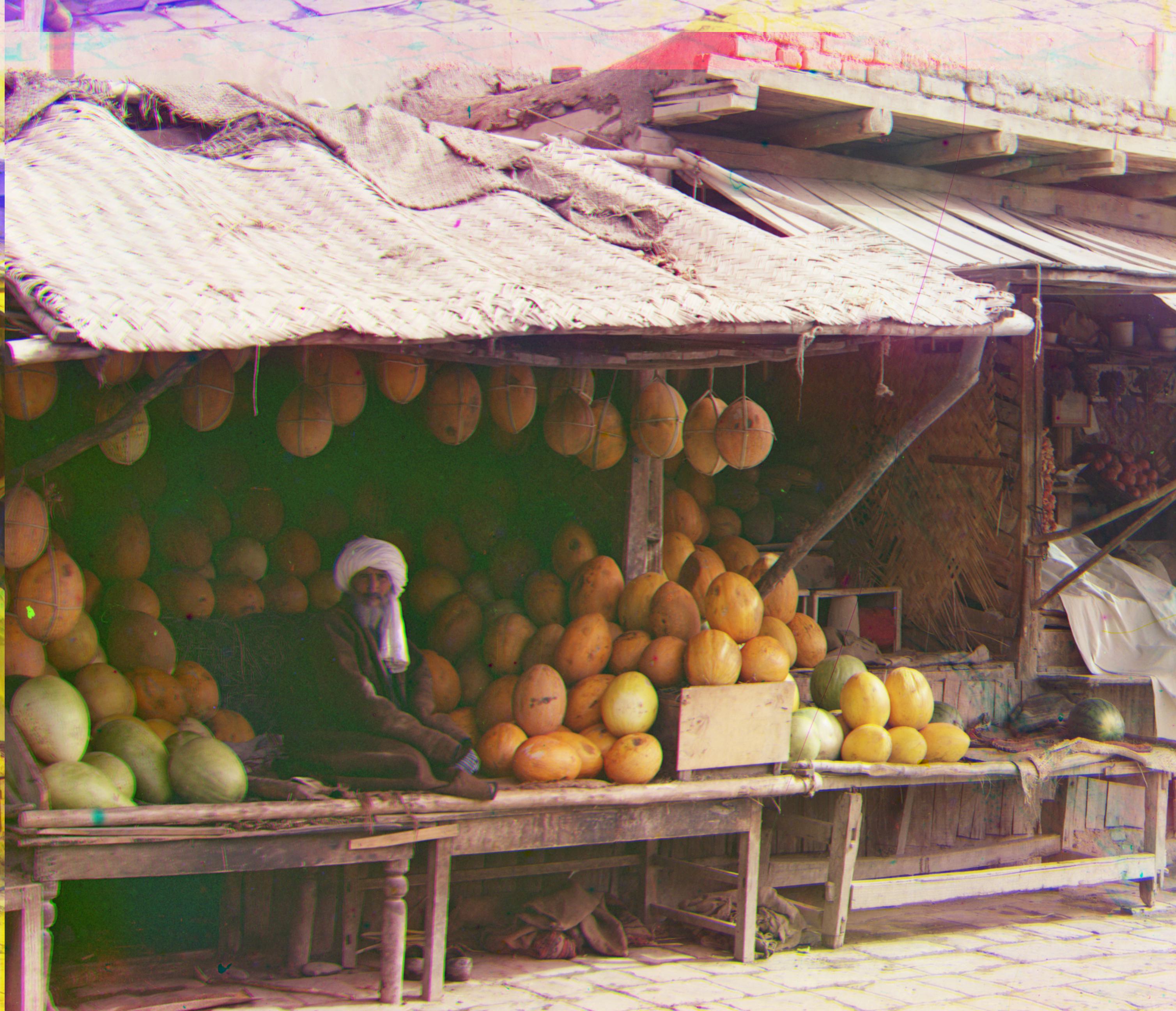
 melons.jpg: G(82, 12), R(178, 12)
|
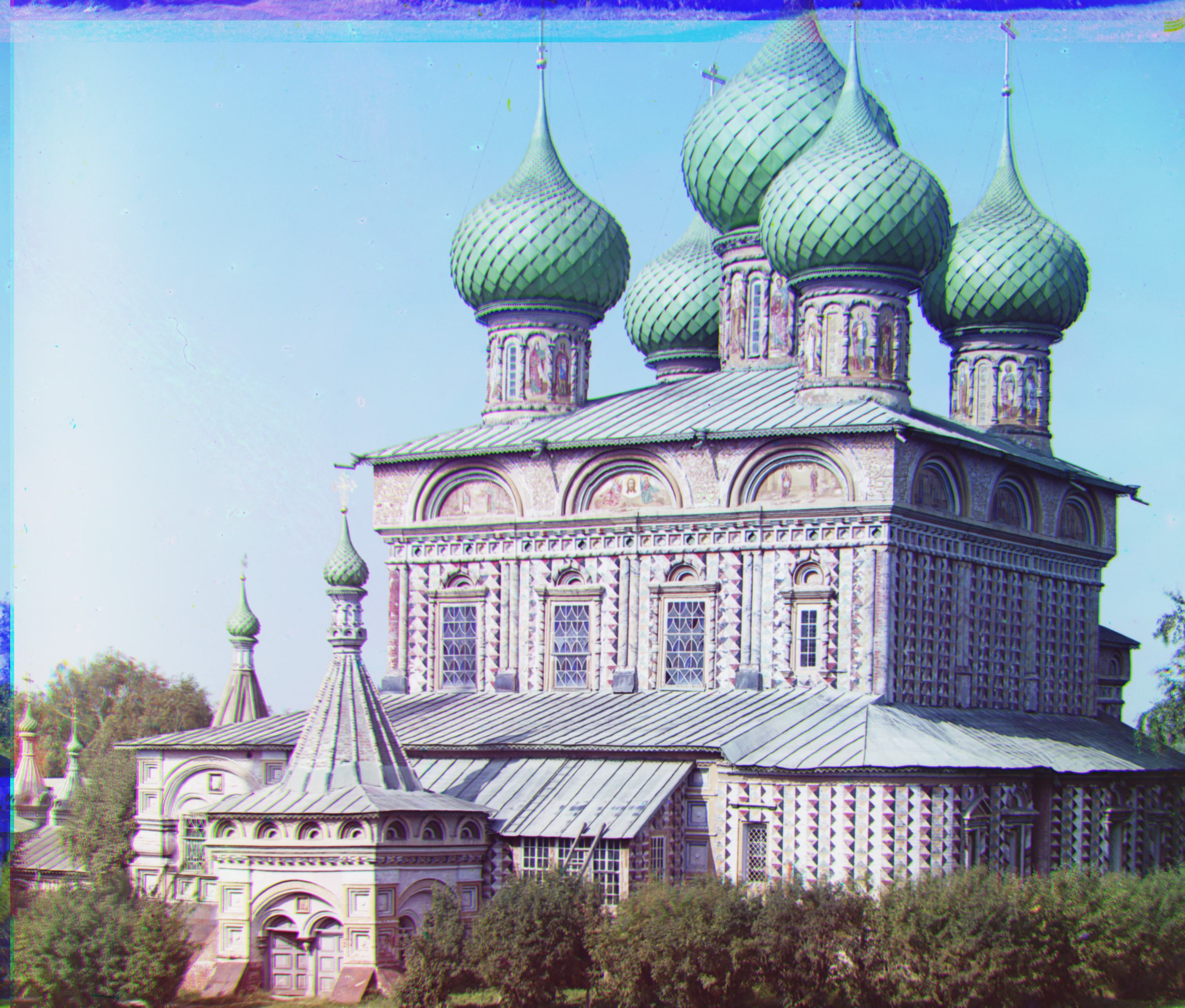
 onion_church.jpg: G(52, 26), R(108, 36)
|
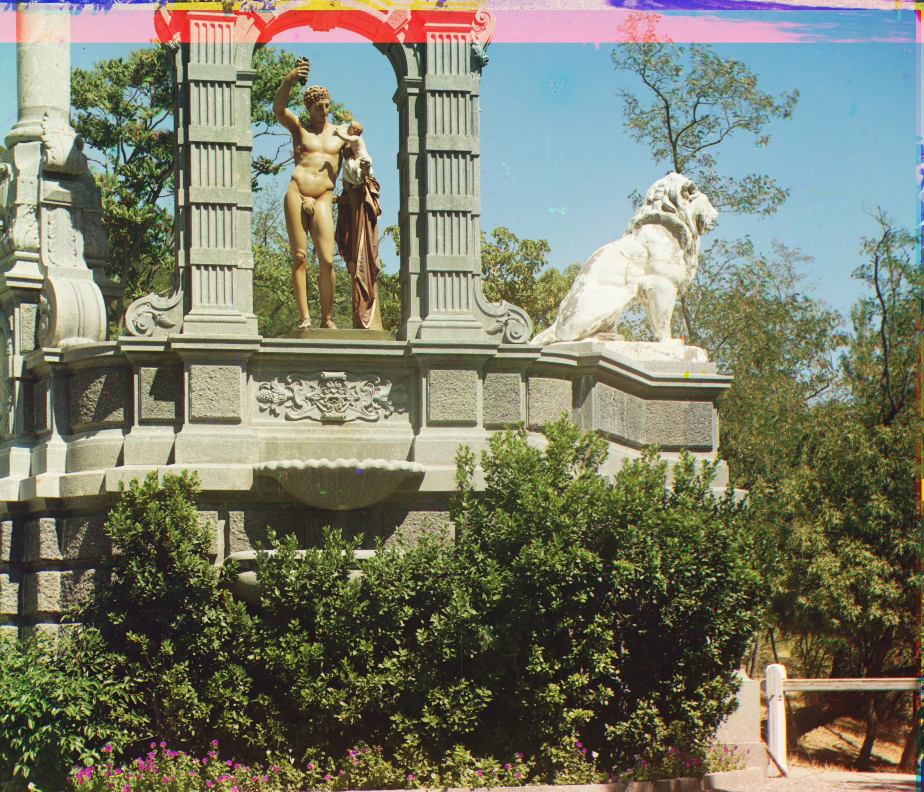
 sculpture.jpg: G(34, -10), R(140, -26)
|
 self_portrait.jpg: G(78, 28), R(176, 36)
|
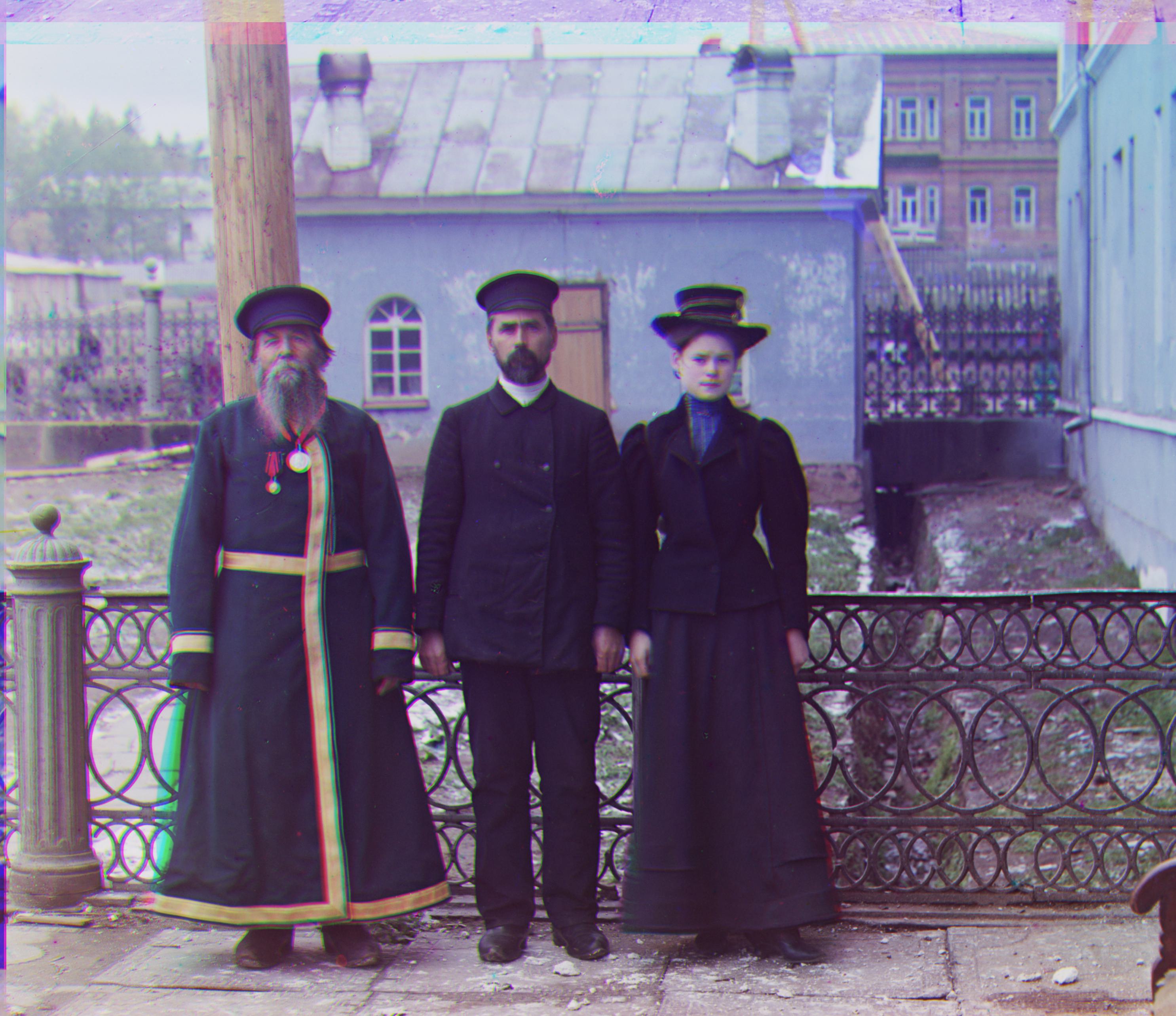
 three_generations.jpg: G(56, 16), R(112, 10)
|
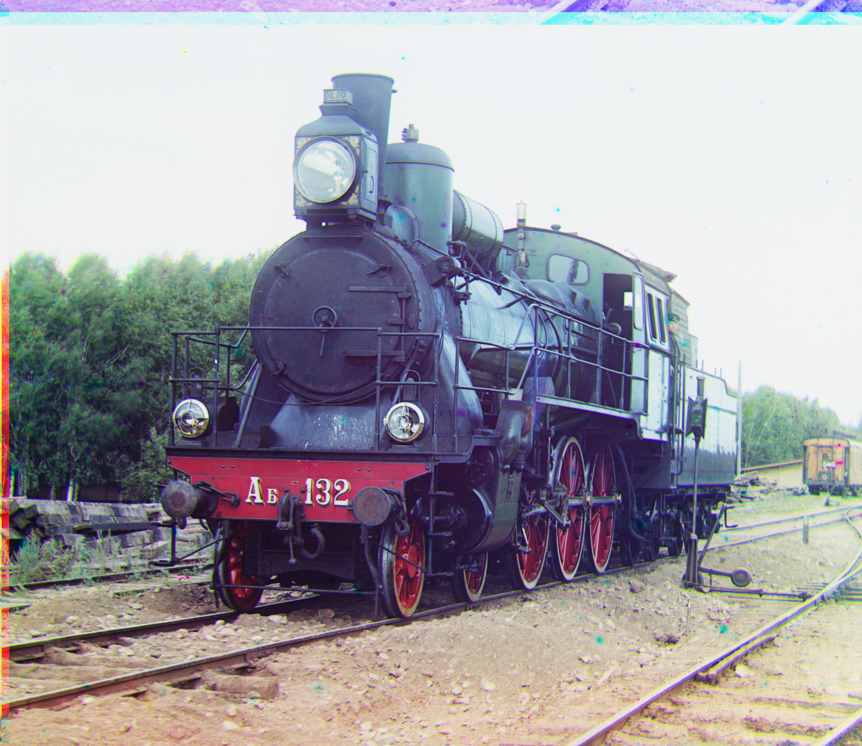
 train.jpg: G(42, 6), R(86, 32)
|
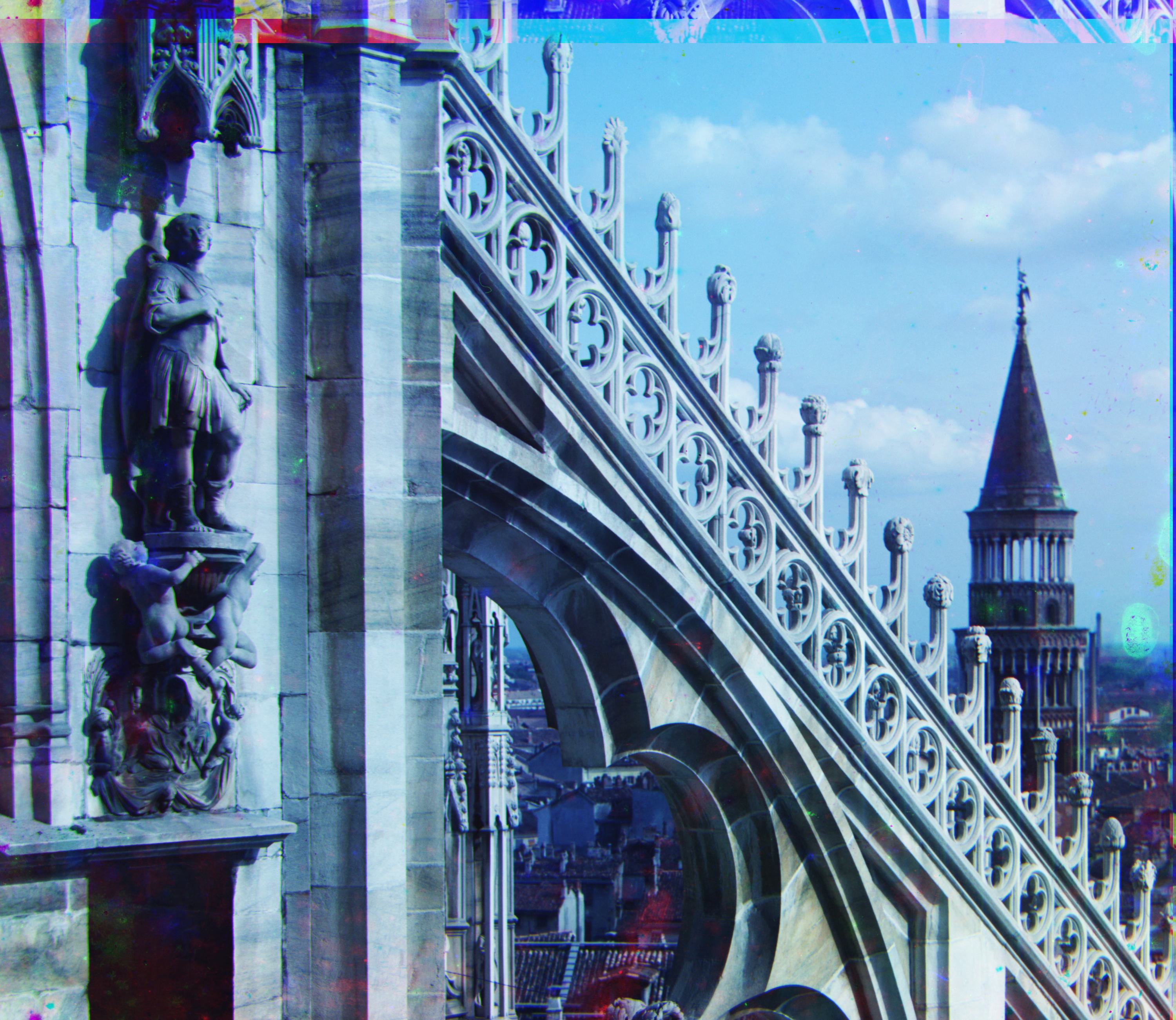
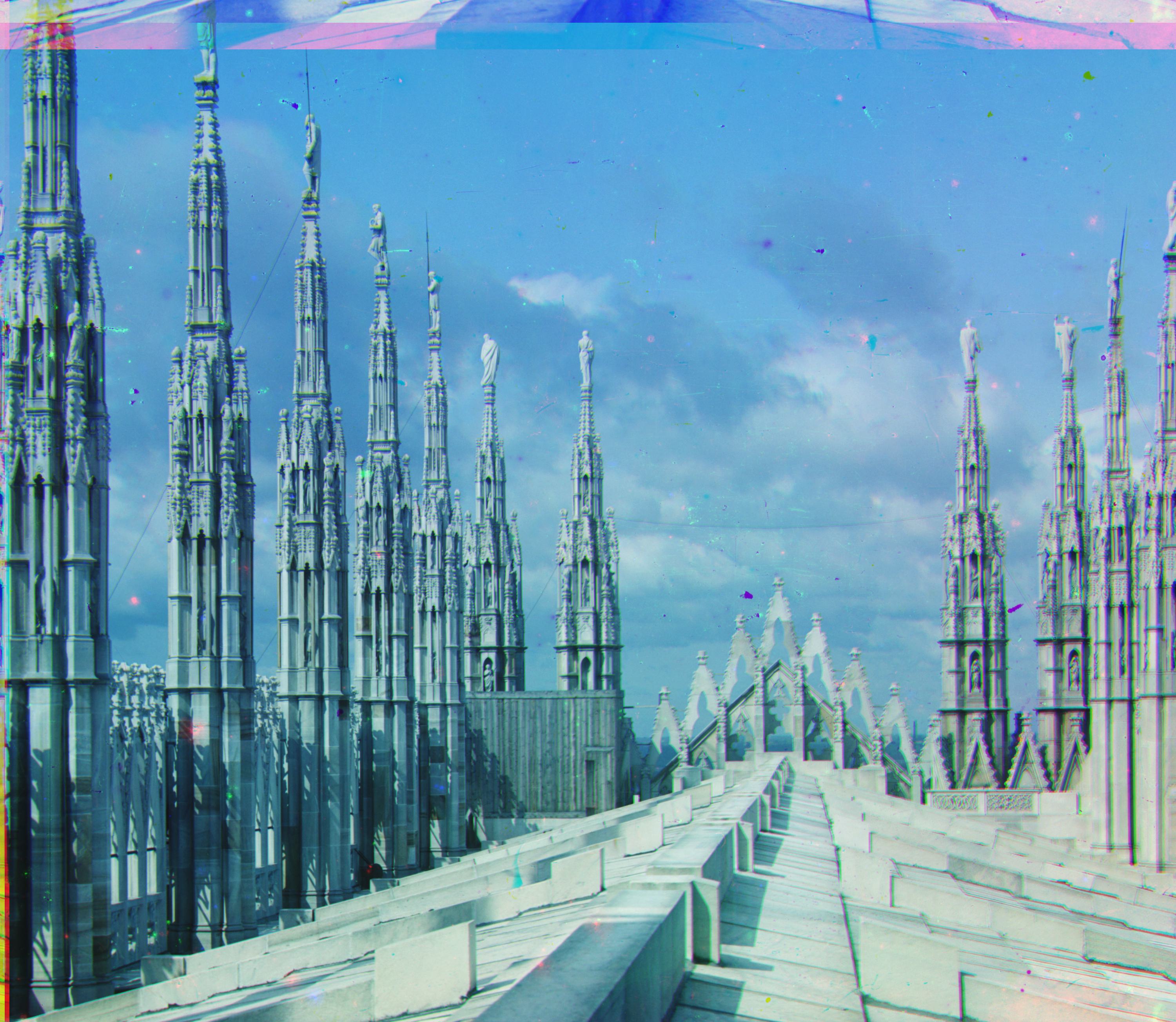
 milane1.jpg: G(48, -8), R(110, -16)
|
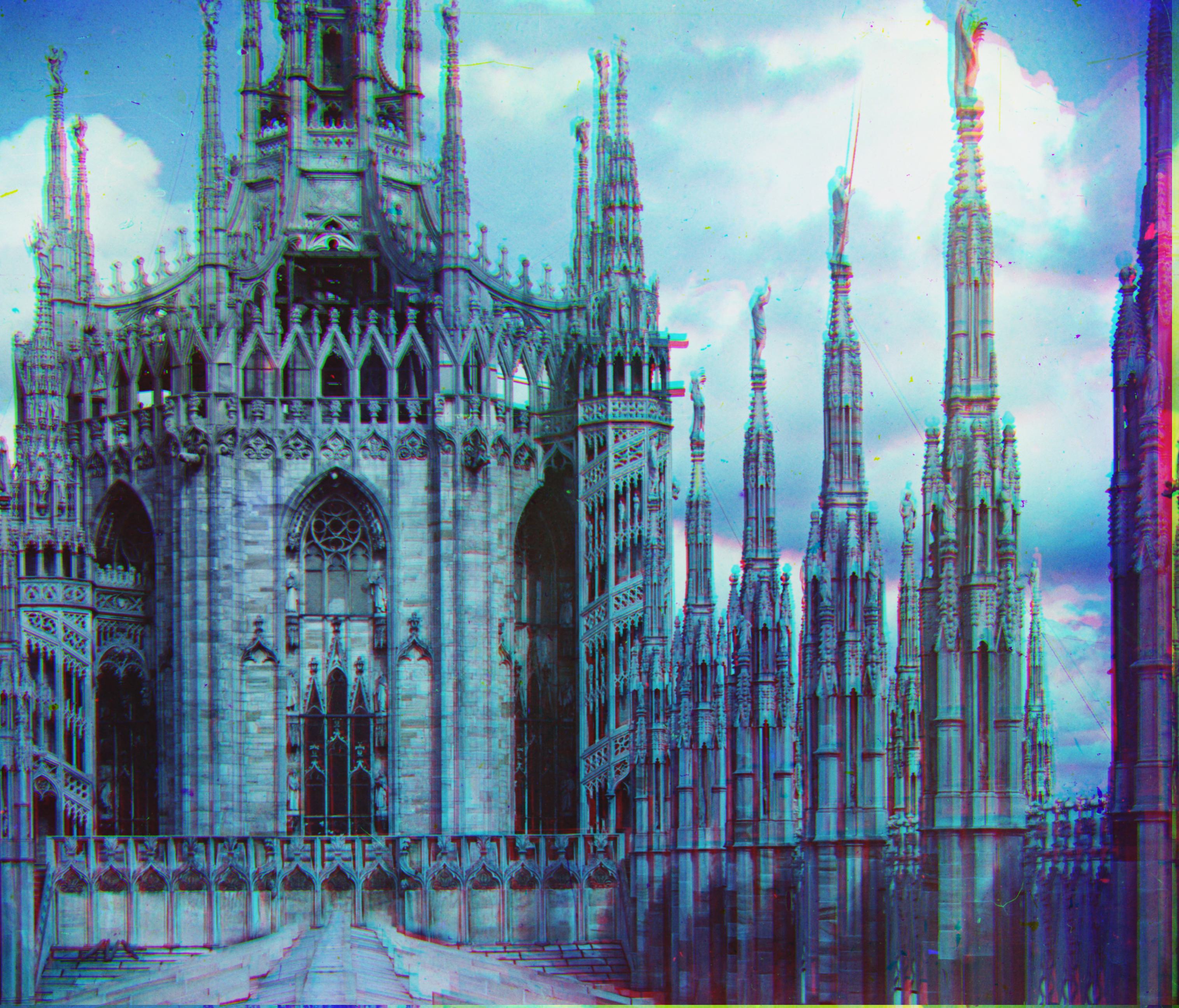
 milane2.jpg: G(58, 12), R(126, 24)
|
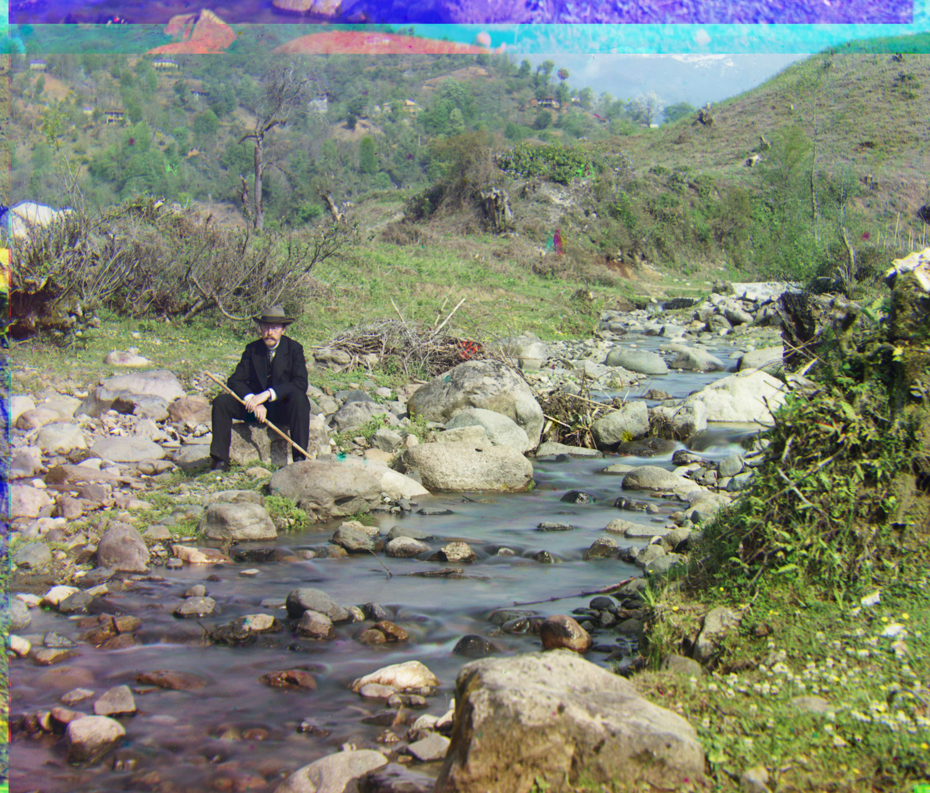
 milane3.jpg: G(-8, -18), R(-8, -54)
|
Most of the issues that I ran into during this project was having the alignment score properly. When working on the single-scale case, I found that all of my images were not aligning properly, even when adding
functionality to take care of cropping black bars and using other features such as edges using scikit-image's Sobel filter function. The actual underlying issue was that I wasn't setting the best alignment score
properly so it was never being updated, meaning that it would stay at the initial alignment and would not give any new displacment vector to use.
When working on the multi-scale case, I had the similar issue where every TIF image would be misaligned. Now that the alignment scoring function was fixed, I tried greatly expanding the search case, which wasn't a viable solution
since it would take over 20 minutes to do 1 pass of the pyramid-based alignment and a small increase in the search space would have virtually no effect. This was where I also tried adding the similar structural scoring metric which did not change anything
but did give an alternative scoring metric I can use. The actual underlying issue was that I was not properly updating my "best" displacement vector in each step of the coarse-to-fine pyramind alignment function. Originally, I
just had the displacement vector be updated as (best_displacement_vector + new_search_space). Since we double the resolution of the current working image after each iteration of the image pyramid, the issue was that as we increased
resolution, the actual search space centered around the best displacement vector was still as if it was in the previous smaller resolution image, so it was ignoring the new pixel information in the newer higher resolution. The
fix was to multiply the displacement vector by 2 to compensate for the doubling in resolution.
Lastly, my initial image pyramid took advantage of OpenCV's pyramid construction function found here: OpenCV Image Pyramid which is not
allowed since we have to construct the pyramid from scratch. I had to adapt the "cv2.PyrDown" function to use scikit-image's functions which was just to apply a blur and downscale the image.
