Overview
The goal of this assignment is to start viewing images in the frequency domain. We can use the various frequencies of the image to show off some cool image processing techniques. For instance, we can extract the low frequencies
of one image and combine it with the high frequencies of another image and create a hybrid. We can amplify the high frequencies of an image to sharpen it and do the inverse to blur it. These are a few examples that we will showcase
in this project.
Section I-I: Finite Difference Operator
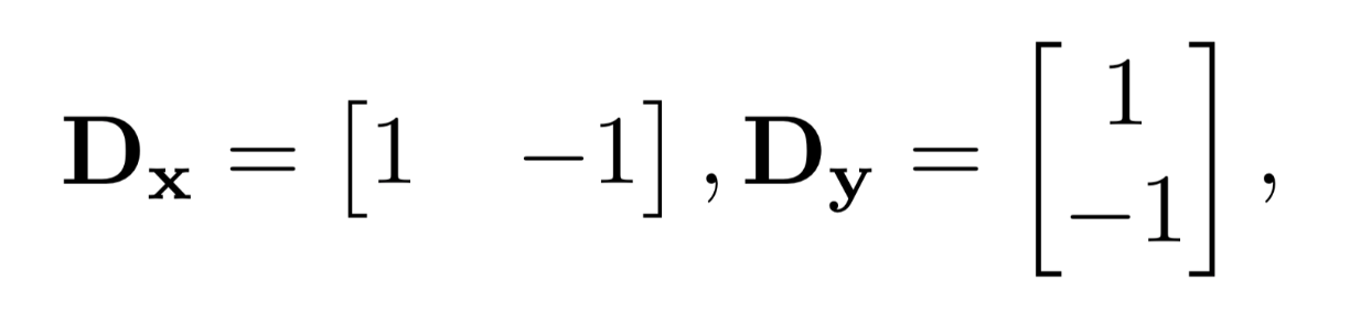
We will begin by using the humble finite difference as our filter in the x and y directions.
We will show the partial derivative in x and y of the cameraman image by convolving the image with finite difference operators D_x and D_y. Next, we will compute and show the gradient magnitude image. To turn this into an edge
image, we will binarize the gradient magnitude image by picking the appropriate threshold (trying to suppress the noise while showing all the real edges).
To achieve this, we first convolve the original image with the differential operators giving us the partial derivatives in the x and y directions. Next, we take the image gradient by computing the square root of the sum of the squared partials.
Lastly, we can binarize the edges by specifying a threshold and if a pixel value meets this threshold, it is at full intensity and zero otherwise.
 Difference Operator
|
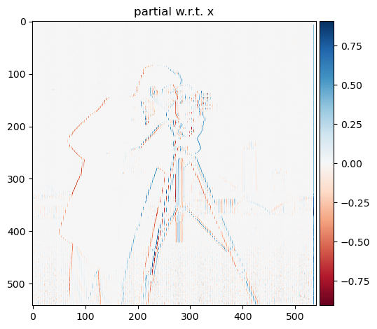 Partial w.r.t. x
|
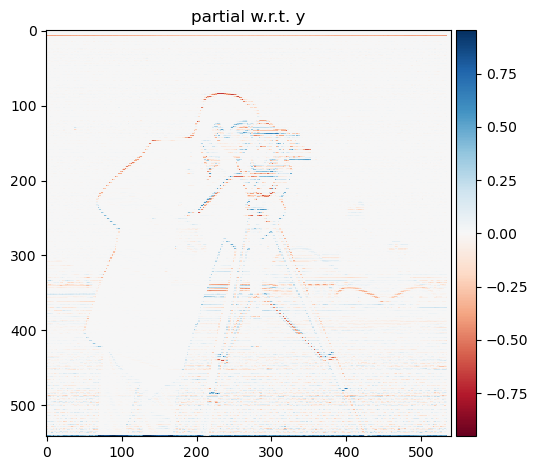 Partial w.r.t. y
|
 Edge Map
|
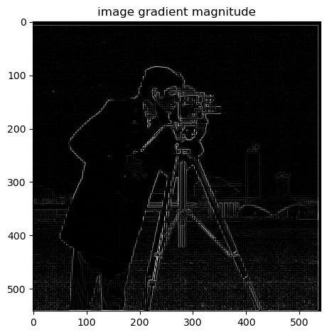 Gradient Map
|
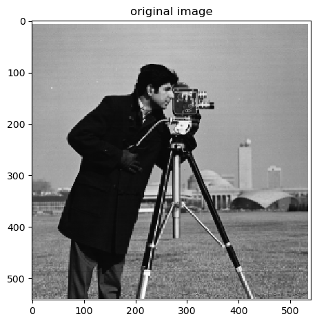 Original Image
Section I-II: Derivative of Gaussian (DoG) Filter
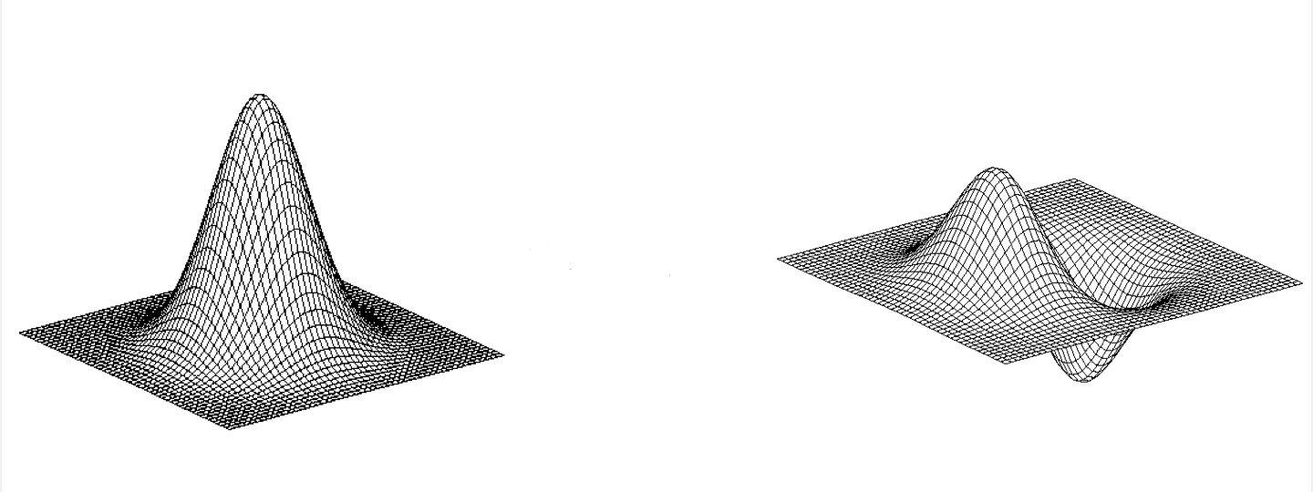
Our previous results show that the images and maps ended up quite noisy. Luckily, we have a smoothing operator handy: the Gaussian filter G. First, we will create a blurred version of the original image by convolving with a
gaussian and repeat the procedure in the previous part. We can achieve this by creating a 2D gaussian filter with cv2.getGaussianKernel() to create a 1D gaussian and then take the outer product with its transpose to get a 2D
gaussian kernel. After convolving the image with this gaussian kernel, we will convolve again using the previous differential operators like in the last section to get a map of the partial derivatives, gradient, and edges.
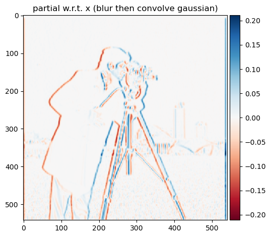 Partial w.r.t. x (filtered)
|
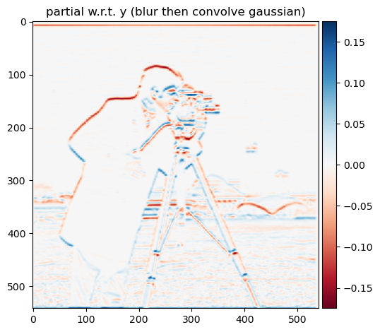 Partial w.r.t. y (filtered)
|
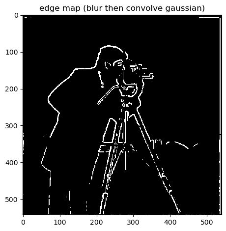 Edge Map (filtered)
|
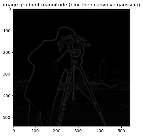 Gradient Map (filtered, a little dark)
|
 Original Image (filtered)
By prefiltering the image, we see the our processed are much smoother and do not contain as much aliasing as the images without the preprocessing. In addition, if we convolve the gaussian filter G with the differential operator
first and then the image, we observe that the results are the same as above with blurring with the gaussian first then taking the differential.
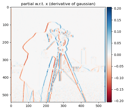 Partial w.r.t. x (DoG)
|
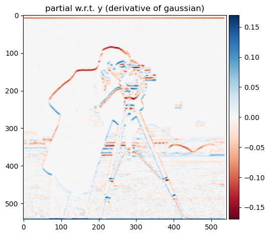 Partial w.r.t. y (DoG)
|
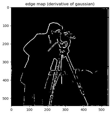 Edge Map (DoG)
|
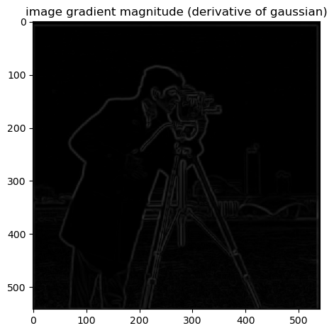 Gradient Map (DoG, a little dark)
|
Section II-I: Image Sharpening
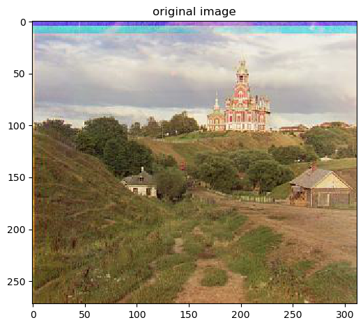
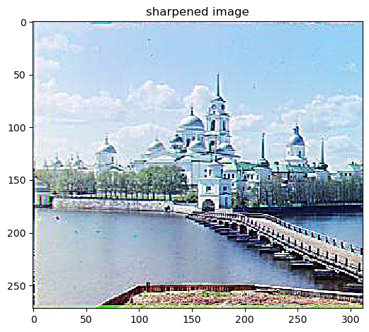
In this section, we will discuss how to "sharpen" an image. Essentially, we want to emphasize the high frequencies of an image to increase detail in certain areas of the image. An image often looks sharper if it has stronger high
frequencies.
To achieve this, we will first separate the image into its 3 separate color channels: R, G, B. Then we convolve each channel with the gaussian filter used previously. We can consider this a low pass filter from now on since it only
retains the low frequencies of the image. Next, we will subtract these low frequencies from the original frequencies: high_frequencies = original_frequencies - low_frequencies. Next, we will add these high frequencies to the original
image multiple by some sharpening factor alpha: sharpened_image = original_frequencies + alpha * high_frequencies (after stacking the 3 channels back together).
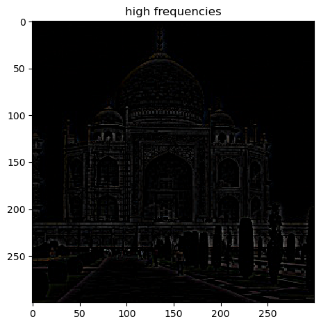 High Frequencies
|
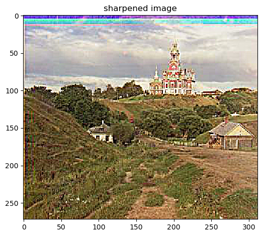
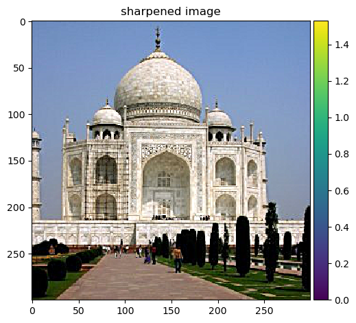 Sharpened, alpha=2, kernel=10, sigma=10/6
|
|
|
|
 Original Image
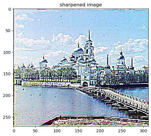
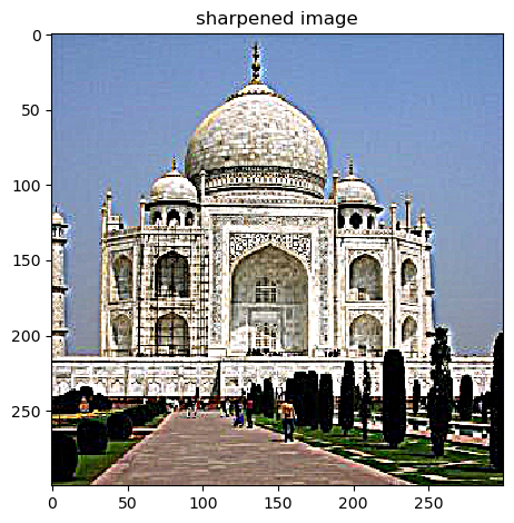 Sharpened, alpha=4, kernel=10, sigma=10/6
|
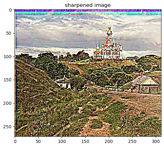
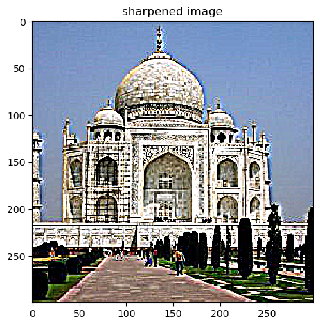 Sharpened, alpha=6, kernel=10, sigma=10/6
|
 Original
|
 Sharpened, alpha=2, kernel=10, sigma=10/6
|
 Sharpened, alpha=4, kernel=10, sigma=10/6
|
 Sharpened, alpha=6, kernel=10, sigma=10/6
|
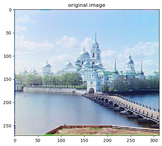 Original
|
 Sharpened, alpha=2, kernel=10, sigma=10/6
|
 Sharpened, alpha=4, kernel=10, sigma=10/6
|
 Sharpened, alpha=6, kernel=10, sigma=10/6
|
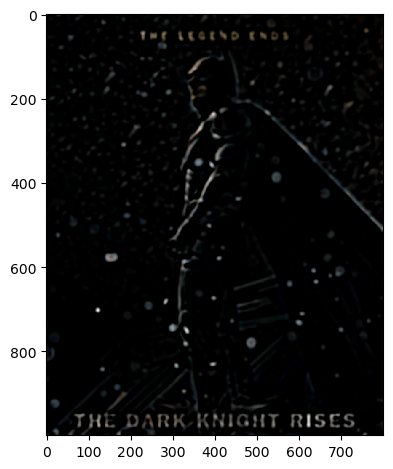
Section II-II: Hybrid Images
In this section, the goal is to create hybrid images using the approach described in the SIGGRAPH 2006 paper by Oliva, Torralba, and Schyns. Hybrid images are static images that change in interpretation as a function of the
viewing distance. The basic idea is that high frequency tends to dominate perception when it is available, but, at a distance, only the low frequency (smooth) part of the signal can be seen. By blending the high frequency
portion of one image with the low-frequency portion of another, you get a hybrid image that leads to different interpretations at different distances.
To achieve this, we first need to get 2 images that we want to combine into a hybrid image. We might need to align both if necessary. First, we will perform a low pass filter on one image, which is just taking the gaussian filter used
previously and blurring the image. Next, we will perform a high pass filter on the second image, which is the processing of sharpening done previously, where we extract the low frequencies using the low pass filter and subtract from
the original image to get the high frequencies (alpha * (image - low_pass_filter(image, kernel_size, sigma))). After we process both images where one is blurred and one is sharpened, we will average both images together and get our
hybrid image.
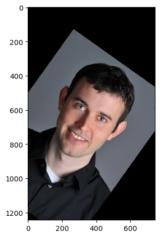 Image 1
|
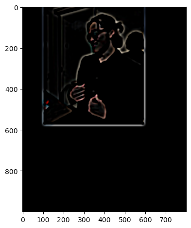
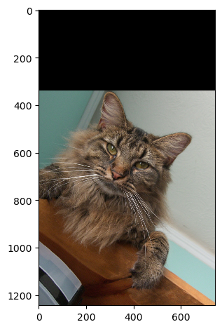 Image 2
|
|
|
|
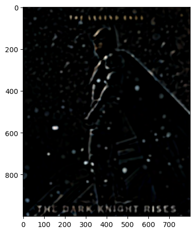
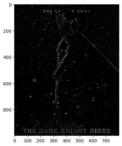
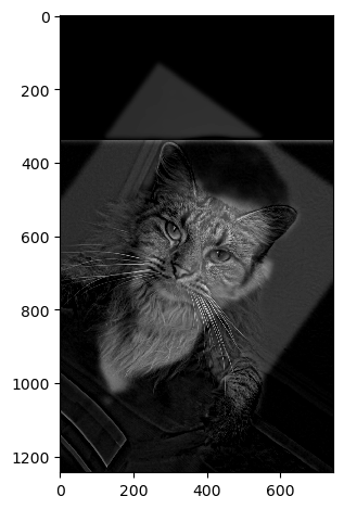 Hybrid Image
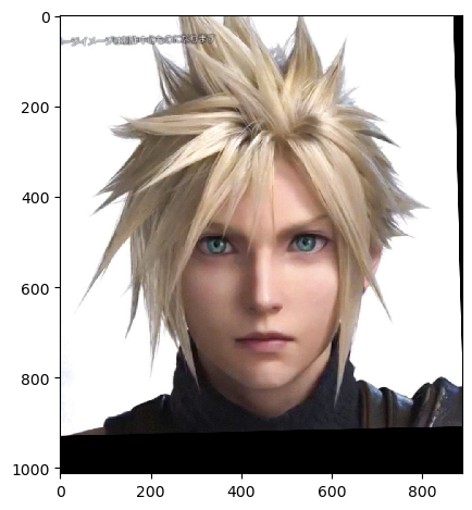 Image 1 (Cloud)
|
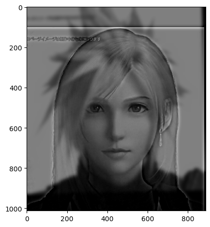
 Image 2 (Tifa)
|
|
|
|
 Hybrid Image
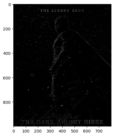
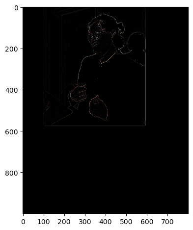
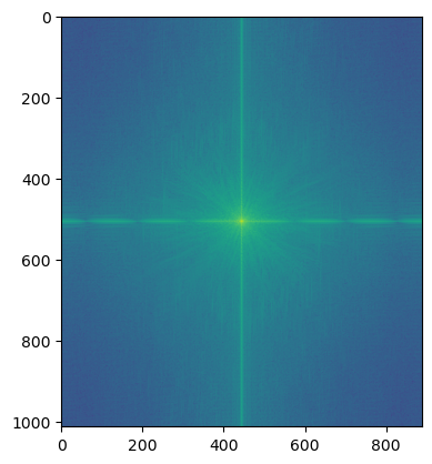
Below is the fourier analysis for (Cloud & Tifa) the original images, filtered images, and the hybrid images above.
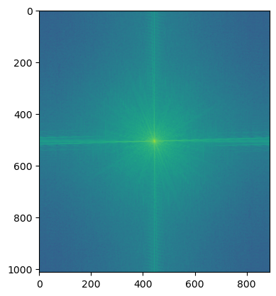 FFT of Image 1
|
 FFT of Image 2
|
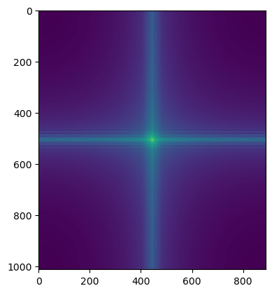 FFT of Low Pass Image (blurred)
|
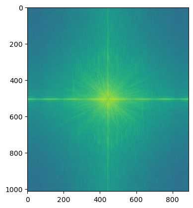 FFT of High Pass Image (sharpened)
|
 FFT of Hybrid Image
|
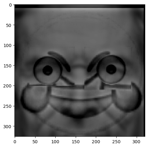
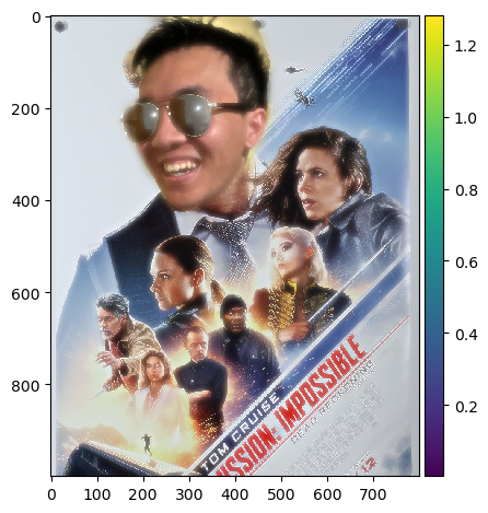
Below is a failed hybrid image attempt where I could not really get a balance between the two where one it is
readable possibly from the photorealistic details of the face contrasted with the clean angles and lower details of the emoji.
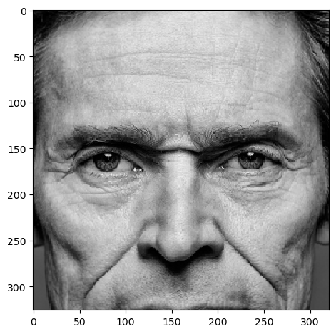 Image 1 (failure), kernel=24, sigma=4
|
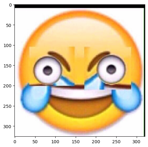 Image 2 (failure), kernel=48, sigma=8
|
|
|
|
 Hybrid Image (failure), alpha=1
Section II-III: Gaussian and Laplacian Stacks
In this section, we will implement Gaussian and Laplacian stacks, which are kind of like pyramids but without the downsampling
To achieve this, we first need to specify how many levels we want our stack to be (the levels of our Laplacian stack will be determined by our Gaussian stack). To implement our Gaussian stack, we will use a list again as our
data structure representing the stack. We will take our original image and make that the first element of our stack. Next, we will iterate by the number of levels that we specified and in each iteration, we will apply a low pass filter
on the image continuously, so with the each iteration, the current image will get blurrier. In each iterator, we will add that blurred image at that level to the list and that will be the image represented at that particular
Gaussian stack level.
Now, that we have our Gaussian stack, we can start creating our Laplacian stack. We will start by iterating
through our Gaussian stack and stop at the second to last level. We will also represent our Laplacian stack
as a list. On each iteration, we will take the current image (at level i) and the next image (at level i + 1) and
then subtract the next image from the current image (laplacian = cur_im - next_im). We will add this image
to our list and that will represent the particular level in the laplacian stack. Lastly, we will add the last
element of the Gaussian stack to our Laplacian stack.
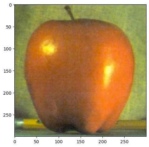 apple: Gaussian Stack 0
|
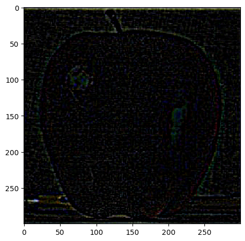 apple: Laplacian Stack 0 (Normalized for Visualization)
|
 apple: Gaussian Stack 1
|
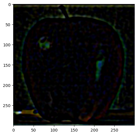 apple: Laplacian Stack 1 (Normalized for Visualization)
|
 apple: Gaussian Stack 2
|
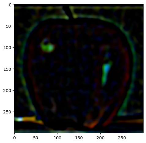 apple: Laplacian Stack 2 (Normalized for Visualization)
|
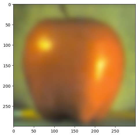 apple: Gaussian Stack 3
|
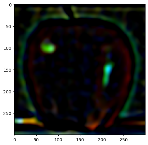 apple: Laplacian Stack 3 (Normalized for Visualization)
|
 apple: Gaussian Stack 4
|
 apple: Laplacian Stack 4 (Normalized for Visualization)
|
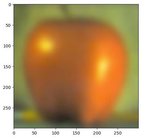
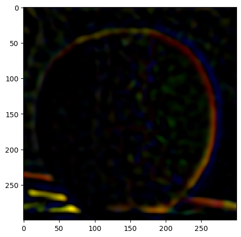
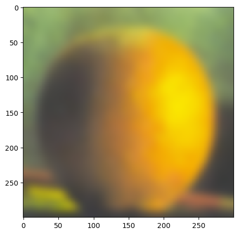
 orange: Gaussian Stack 0
|
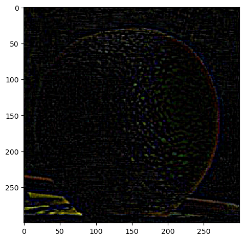 orange: Laplacian Stack 0 (Normalized for Visualization)
|
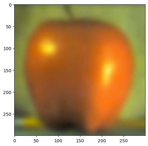
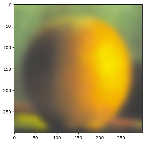
 orange: Gaussian Stack 1
|
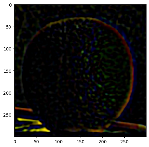 orange: Laplacian Stack 1 (Normalized for Visualization)
|
 orange: Gaussian Stack 2
|
 orange: Laplacian Stack 2 (Normalized for Visualization)
|
 orange: Gaussian Stack 3
|
 orange: Laplacian Stack 3 (Normalized for Visualization)
|
 orange: Gaussian Stack 4
|
 orange: Laplacian Stack 4 (Normalized for Visualization)
|
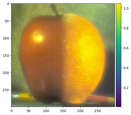
Section II-IV: Multiresolution Blending
A cool thing we can do with gaussian and laplacian stacks is that we can blend images together. However,
if we want to put one half of the apple and one half of the orange together, we find that there is still a
clear seam down the middle. In the pyramid case the downsampling/blurring/upsampling steps ends up blurring
the abrupt seam proposed in this algorithm, but we are using stacks so these steps do not apply.
 Initial Oraple
|
To remedy this, we will use a mask. The Gaussian blurring of the mask in the pyramid will smooth out the
transition between the two images. For the vertical or horizontal seam, your mask will simply be a step function
of the same size as the original images.
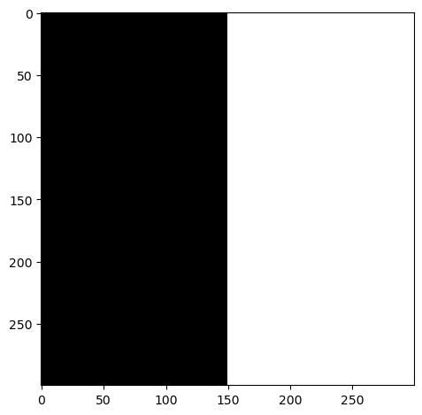 Vertical Seam Mask
|
 Oraple using mask
|
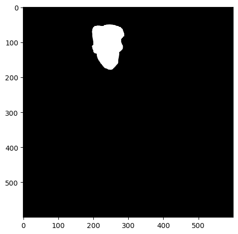
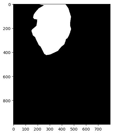
To achieve this, we will take our two images again and create gaussian and laplacian stacks for both. Next,
we will create our mask, which is an image of the same dimensions where each pixel is either 0 (black) or 1 (white)
and the transition from white to black will determine where the transitions between the two images will happen.
We then create a gaussian stack for the mask, so now we have a total of 3 gaussian stacks and 2 laplacian stacks
for the two images we're blending.
Now that we have all our stacks (which all have the same number of levels), we will iterate through the number of levels.
In each iteration i (or level i), we will take the image at that level in the 2 laplacian stacks
for the images we want to blend, and the image in the gaussian stack for the mask and perform this operation:
(1 - mask_gaussian[i]) * laplacian_image1[i] + mask_gaussian[i] * laplacian_image2[i]
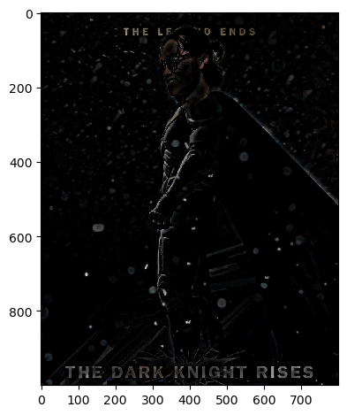
We will do this calculation at each iteration and add each up to make the final blended image:
blended = (1 - mask_gaussian) * laplacian_image1 + mask_gaussian * laplacian_image2
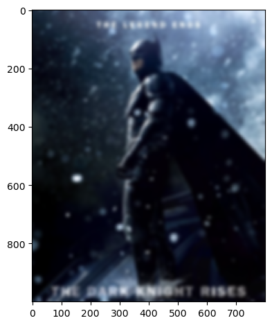
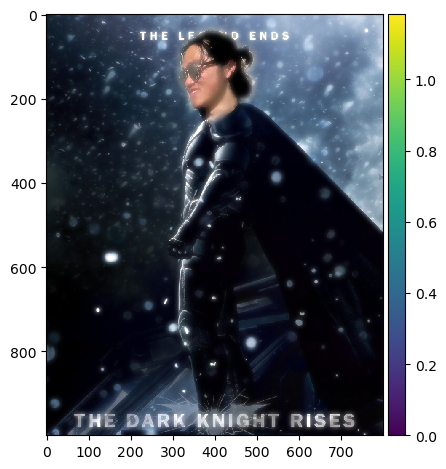
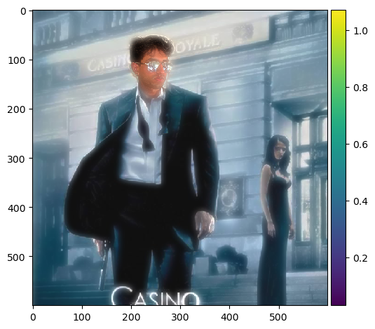
Now my roommates can fulfill their action movie star dreams!
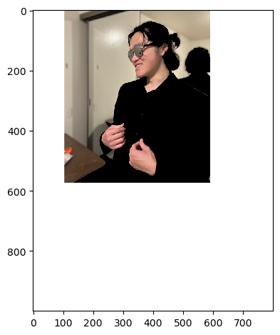 Image 1
|
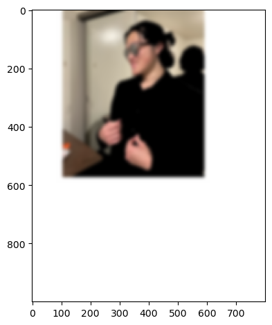
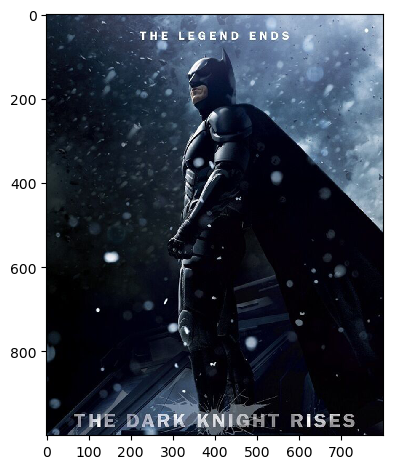 Image 2
|
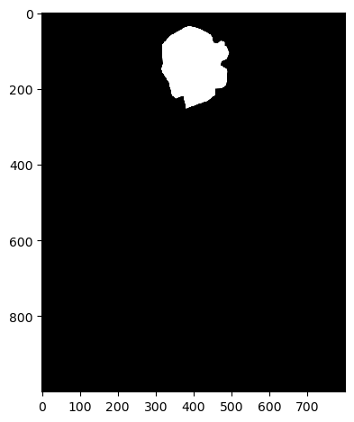 Mask
Mask
|
 Blended Image
|
Laplacian stacks for blended image above.
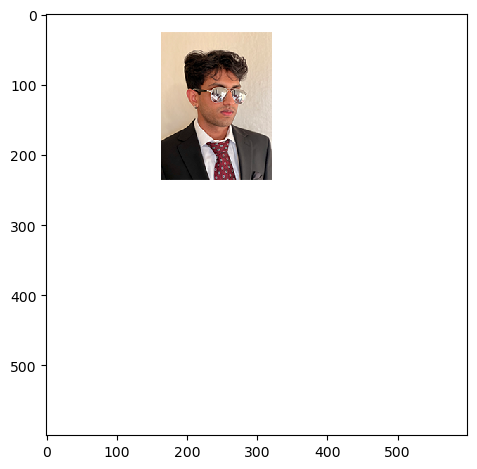 Image 1
|
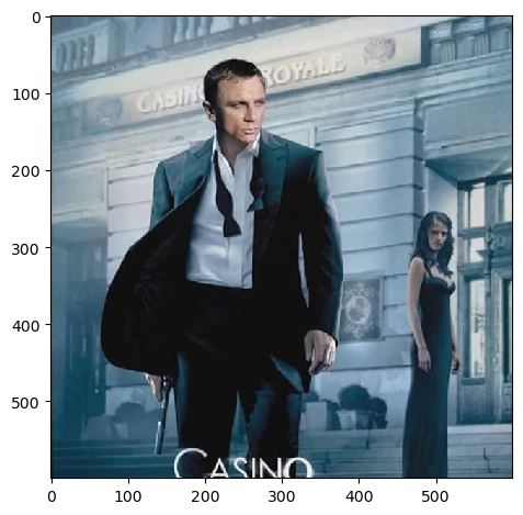 Image 2
|
 Mask
Mask
|
 Blended Image
|
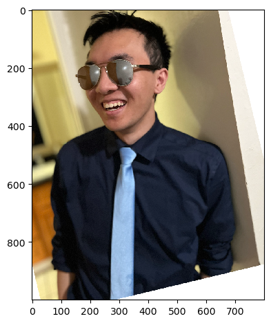 Image 1
|
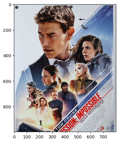 Image 2
|
 Mask
Mask
|
 Blended Image
|