Overview
In this assignment, we will explore diffusion models, implement diffusion sampling loops, and use them for other tasks such as inpainting and
creating optical illusions. We will also train our own diffusion model on the MNIST dataset.
Part A: The Power of Diffusion Models!
Part A - Section 0: Setup
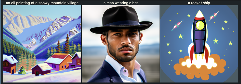
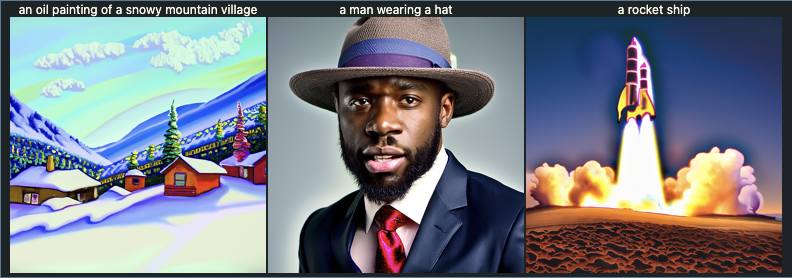
First, we need to install our dependencies, load the models, seed our work, and test the model with the provided sampling loops. We are using seed 180.
 3 Prompts - 20 Inference Steps
|
 3 Prompts - 40 Inference Steps
|
Part A - Section 1: Sampling Loops
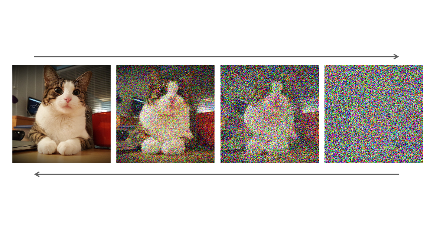
Starting with a clean image, x0, we can iteratively add noise to an image, obtaining progressively more and more noisy versions of the
image, xt, until we're left with basically pure noise at timestep t = T. When t = 0, we have a clean image, and for
larger t more noise is in the image. A diffusion model tries to reverse this process by denoising the image. By giving a diffusion model a
noisy xt and the timestep t, the model predicts the noise in the image. With the predicted noise, we can either
completely remove the noise from the image, to obtain an estimate of x0, or we can remove just a portion of the noise,
obtaining an estimate of xt-1, with slightly less noise. To generate images from the diffusion model (sampling), we
start with pure noise at timestep T sampled from a gaussian distribution, which we denote xT. We can then predict and
remove part of the noise, giving us xT-1. Repeating this process until we arrive at x0 gives us a clean image.
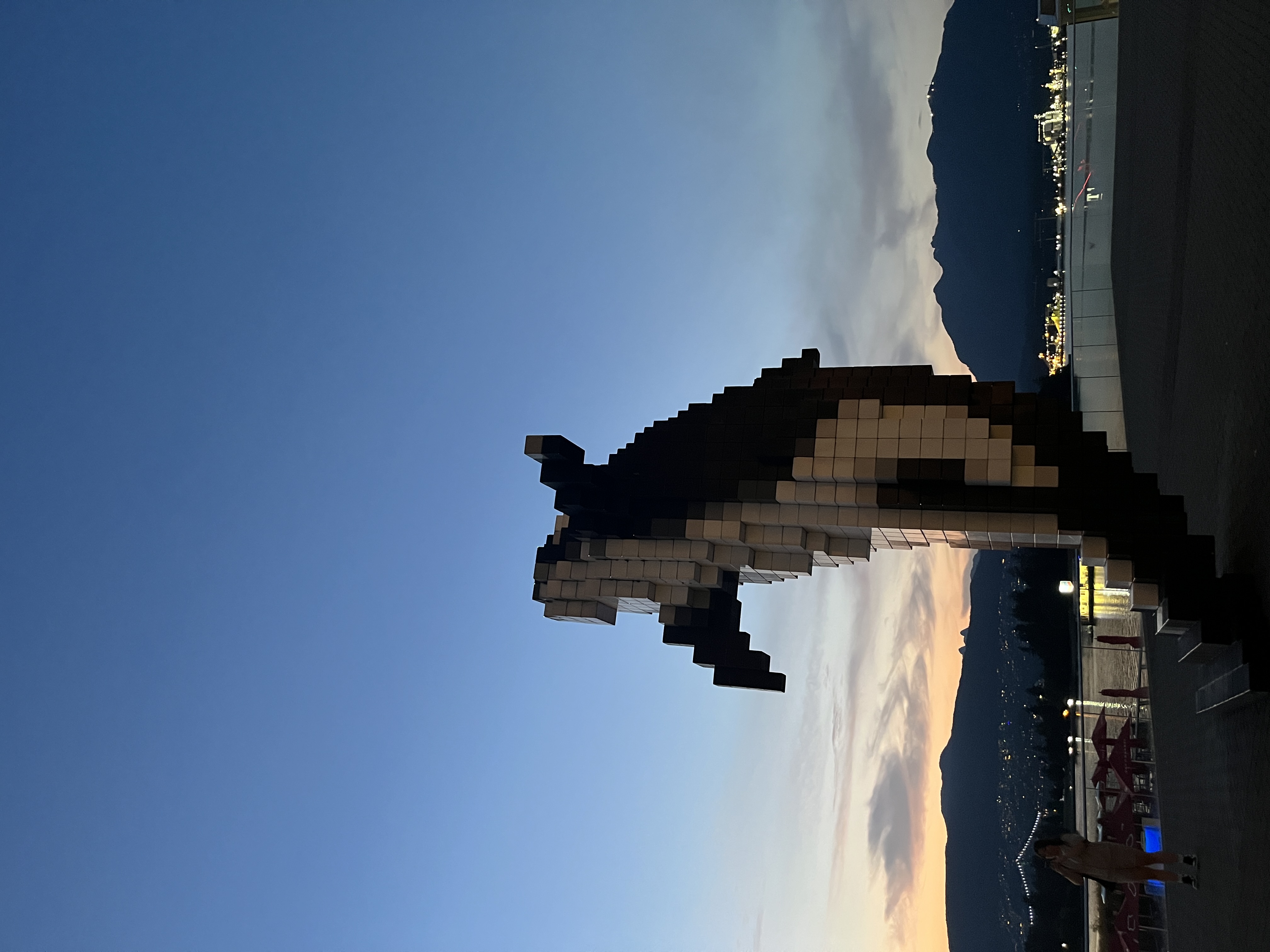
For stage 1, we will use a test image, but resize it down to a 64x64 image and convert it to a (1, 3, 64, 64) tensor.
 Test Image
|
Part A - Section 1.1: Implementing the Forward Process
The forward process can be defined by this equation:
\[
x_t = \sqrt{\bar{\alpha}}x_0 + \sqrt{1 - \bar{\alpha_t}}\epsilon \enspace where \enspace \epsilon \sim N(0,1)
\]
That is, given a clean image x0, we get a noisy image xt at timestep t by sampling from a Gaussian
with mean $$\sqrt{\bar{\alpha}}x_0$$ and variance $$ (1 - \bar\alpha_t). $$ Note that the forward process is not just adding noise -- we also scale the image.
Part A - Section 1.2: Classical Denoising
We will try to remove noise from the image, using Gaussian blur filtering, but this will be impossible for the most part.
Part A - Section 1.3: Implementing One Step Denoising
Instead of blurring, we'll use a pretrained diffusion model to denoise. The actual denoiser can be found at stage_1.unet. We can estimate this with
\[
image \enspace - \enspace \sqrt{1 - \bar{\alpha_t}} \enspace * \enspace (noise\:estimate) / \sqrt{\bar{\alpha_t}}
\]
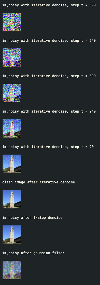
Part A - Section 1.4: Implementing Iterative Denoising
We saw that the denoising UNet does a much better job of projecting the image onto the natural image manifold, but it does get worse as you add
more noise. This makes sense, as the problem is much harder with more noise! But diffusion models are designed to denoise iteratively. We can speed
up this iterative process by skipping steps.
To skip steps we can create a list of timesteps that we'll call strided_timesteps, which will be much shorter than the full list of 1000
timesteps. strided_timesteps[0] will correspond to the noisiest image (and thus the largest t) and strided_timesteps[-1] will correspond
to a clean image (and thus t = 0). One simple way of constructing this list is by introducing a regular stride step (e.g. stride of 30
works well). On the ith denoising step we are at t = strided_timesteps[i], and want to get to t' = strided_timesteps[i+1] (from more noisy to less noisy). To actually do this, we have the following formula:
\[
x_{t'} = \frac{\sqrt{\bar\alpha_{t'}}\beta_t}{1 - \bar\alpha_t} x_0 +
\frac{\sqrt{\alpha_t}(1 - \bar\alpha_{t'})}{1 - \bar\alpha_t} x_t +
v_\sigma
\]
xt is your image at timestep t
xt' is your noisy image at timestep t' where t' < t (less noisy)
is defined as alphas_cumprod
x0 is our current estimate of the clean image
Part A - Section 1.5: Diffusion Model Sampling
We can use the iterative_denoise function is to generate images from scratch. We can do this by setting i_start = 0 and passing in random noise. This effectively denoises pure noise.
 Sample 1
|
 Sample 2
|
 Sample 3
|
 Sample 4
|
 Sample 5
|
Part A - Section 1.6: Classifier Free Guidance
You may have noticed that some of the generated images in the prior section are not very good. We can improve the output with Classifer Free Guidance
(CFG). We define a new noise estimate
where γ controls the strength of CFG. Notice that for γ = 0, we get an unconditional noise estimate, and for γ = 1 we
get the conditional noise estimate. The magic happens when γ > 1.
 Sample 1
|
 Sample 2
|
 Sample 3
|
 Sample 4
|
 Sample 5
|
Part A - Section 1.7: Image-to-image Translation
In Section 1.4, we take a real image, add noise to it, and then denoise. This effectively allows us to make edits to existing images. The
more noise we add, the larger the edit will be. This works because in order to denoise an image, the diffusion model must to some extent
"hallucinate" new things -- the model has to be "creative." Another way to think about it is that the denoising process "forces" a noisy image
back onto the manifold of natural images. Here, we're going to take the original test image, noise it a little, and force it back onto the image
manifold without any conditioning. Effectively, we're going to get an image that is similar to the test image (with a low-enough noise level).
 campanile
|
 i_start = 1
|
 i_start = 3
|
 i_start = 5
|
 i_start = 7
|
 i_start = 10
|
 i_start = 20
|
 car
car
|
 i_start = 1
|
 i_start = 3
|
 i_start = 5
|
 i_start = 7
|
 i_start = 10
|
 i_start = 20
|
 statue
|
|
 i_start = 1
|
 i_start = 3
|
 i_start = 5
|
 i_start = 7
|
 i_start = 10
|
 i_start = 20
|
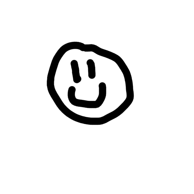
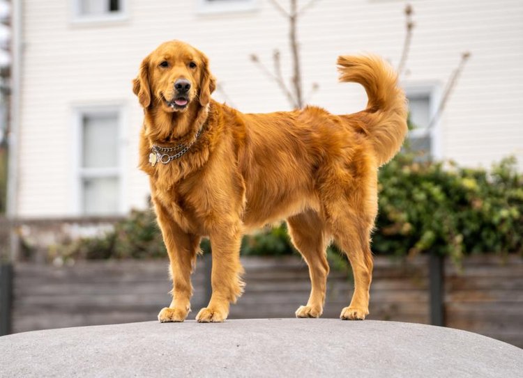
Part A - Section 1.7.1: Editing Hand-Drawn and Web Images
 avocado
|
|
 i_start = 1
|
 i_start = 3
|
 i_start = 5
|
 i_start = 7
|
 i_start = 10
|
 i_start = 20
|
 face
face
|
|
 i_start = 1
|
 i_start = 3
|
 i_start = 5
|
 i_start = 7
|
 i_start = 10
|
 i_start = 20
|
 sword
sword
|
|
 i_start = 1
|
 i_start = 3
|
 i_start = 5
|
 i_start = 7
|
 i_start = 10
|
 i_start = 20
|
 dog
dog
|
|
 i_start = 1
|
 i_start = 3
|
 i_start = 5
|
 i_start = 7
|
 i_start = 10
|
 i_start = 20
|
Part A - Section 1.7.2: Inpainting
Given an image xorig, and a binary mask m, we can create a new image that has the same content where m is 0, but new content wherever
m is 1. To do this, we can run the diffusion denoising loop. But at every step, after obtaining xt, we "force" xtto have the
same pixels as xorig where m is 0:
Part A - Section 1.7.3: Text-Conditional Image-to-image Translation
We will do the same thing as Section 1.7, but guide the projection with a text prompt. We will use the prompt "a rocket ship".
 campanile
|
 i_start = 1
|
 i_start = 3
|
 i_start = 5
|
 i_start = 7
|
 i_start = 10
|
 i_start = 20
|
 car
car
|
 i_start = 1
|
 i_start = 3
|
 i_start = 5
|
 i_start = 7
|
 i_start = 10
|
 i_start = 20
|
 statue
|
 i_start = 1
|
 i_start = 3
|
 i_start = 5
|
 i_start = 7
|
 i_start = 10
|
 i_start = 20
|
Part A - Section 1.8: Visual Anagrams
We can create optical illusions with diffusion models, where the image looks like one image right side up, but a different image upside down.
We will denoise an image at step t to get a noise estimate. At the same time we will flip the image upside down and get another noise estimate.
We flipped the second noise estimate to make it right side up and then average the two estimates. We then do a reverse diffusion step with the new
averaged noise estimate:
 (old man + people around campfire) anagram
|
 anagram flipped
 (mean wearing hat + snowy mountain village) anagram
|
 anagram flipped
 (skull + dog) anagram
|
 anagram flipped
|
Part A - Section 1.9: Hybrid Images
In order to create hybrid images with a diffusion model we can use a similar technique as in Section 1.8. We will create a composite noise estimate , by estimating the noise with two different text prompts, and then combining low frequencies from one noise estimate with high frequencies of the other. The algorithm is:
 skull + waterfall
|
 dog + almafi cost
|
 rocket ship + pencil
|
Part B: Diffusion Models from Scratch!
Part B - Section 1: Training a Single-Step Denoising UNet
Given a noisy image z, we aim to train a denoiser DΘ such that it maps z to a clean image x.
To do so, we can optimize over an L2 loss:
Part B - Section 1.1: Implementing the UNet
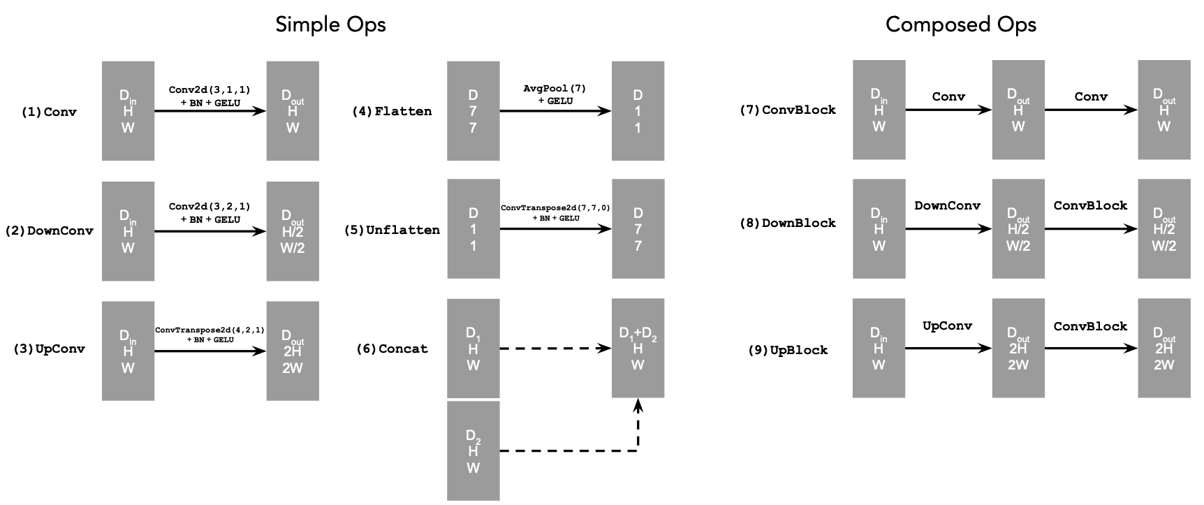
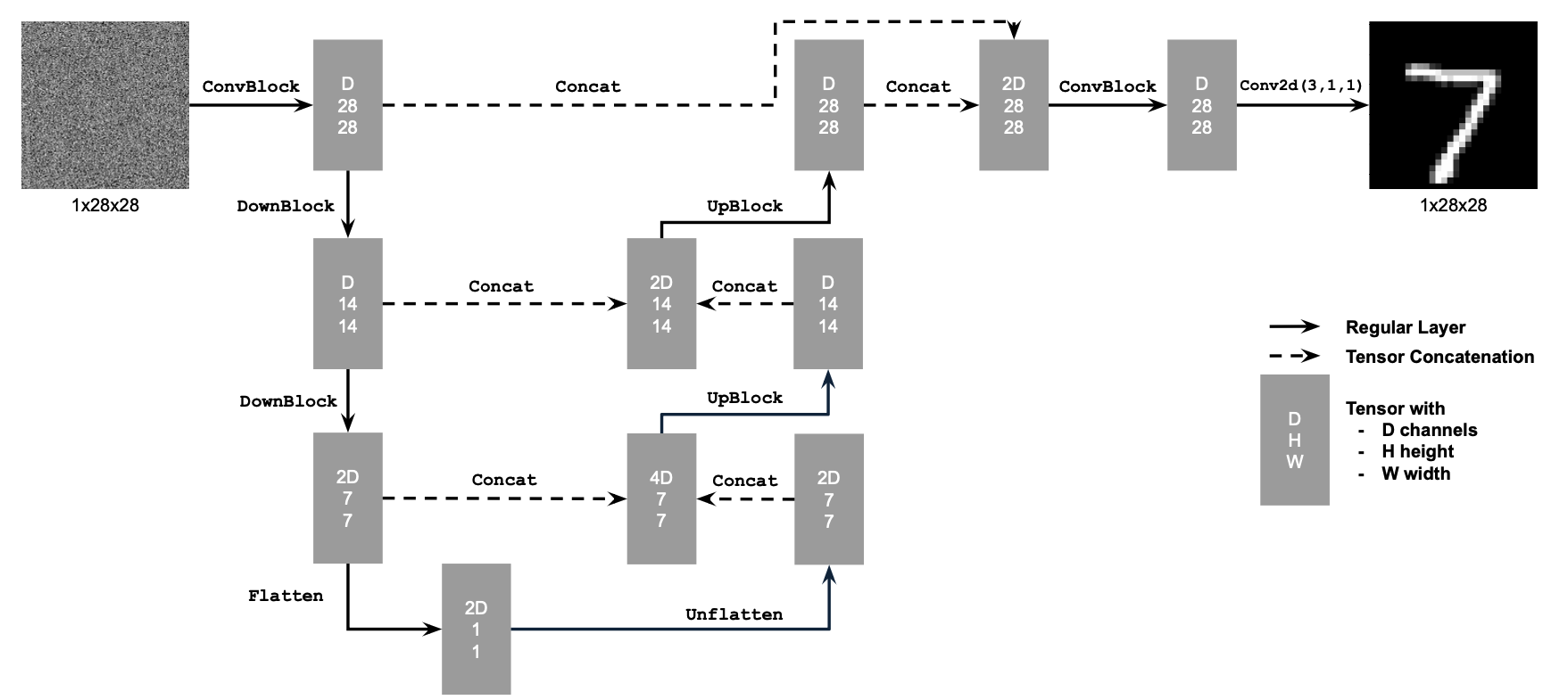
 UNet Operations
|
Our UNet will comprised of various simple and composed operations. We can implement these operations' forward passes as building blocks for our net.
Conv - Run a 2D batch normalization on a 2D convolution with stride length 1, then run a GELU function on that batch
DownConv - Run a 2D batch normalization on a 2D convolution with stride length 2, then run a GELU function on that batch
UpConv - Run a 2D batch normalization on a 2D convolution with stride length 2 and input padding, then run a GELU function on that batch
Flatten - Run 2D average pooling on tensor with kernel size 7
Unflatten - Run a 2D transposed convolution with kernel size 7 and stride length 1
ConvBlock - Call our previous 'Conv' operation on the tensor twice
DownBlock - Run the 'ConvBlock' operation on the 'DownConv' operation
UpBlock - Run the 'ConvBlock' operation on the 'UpConv' operation
 Unconditional
|
For the unconditional UNet, the order of operations will be \[DownBlock \rightarrow DownBlock \rightarrow Flatten \rightarrow Unflatten \rightarrow
UpBlock \rightarrow UpBlock \rightarrow Conv, \]
where we have ConvBlock in DownBlock and UpBlock.
Part B - Section 1.2: Using the UNet to Train a Denoiser
To train our denoiser, we need to generate training data pairs of (z,x), where each is a clean MNIST digit. For each training batch,
we can generate z from x using the the following noising process:
 Noising Process
|
Part B - Section 1.2.1: Training
Lets load our MNIST dataset and initialize our model, optimizer, loss function, and hyperparameters:
Batch Size is 256
5 Epochs
Learning Rate is 1e-4
Sigma is 0.5
128 Hidden Dimensions
For each epoch, we will go through the training dataset, add noise to our clean digit, predict the denoised output using the model, then run the
loss function on the prediction and label.
 After 1 Epoch
|
 After 5 Epochs
|
 Training Loss Over Training Steps
|
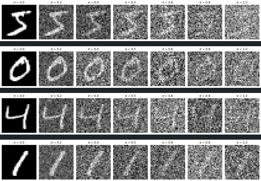
Part B - Section 1.2.2: Out-of-Distribution Testing
The model was trained with sigma value 0.5. Lets see the results with varying sigma values.
 Out-of-Distribution Sigma Values
|
Part B - Section 2: Training a Diffusion Model
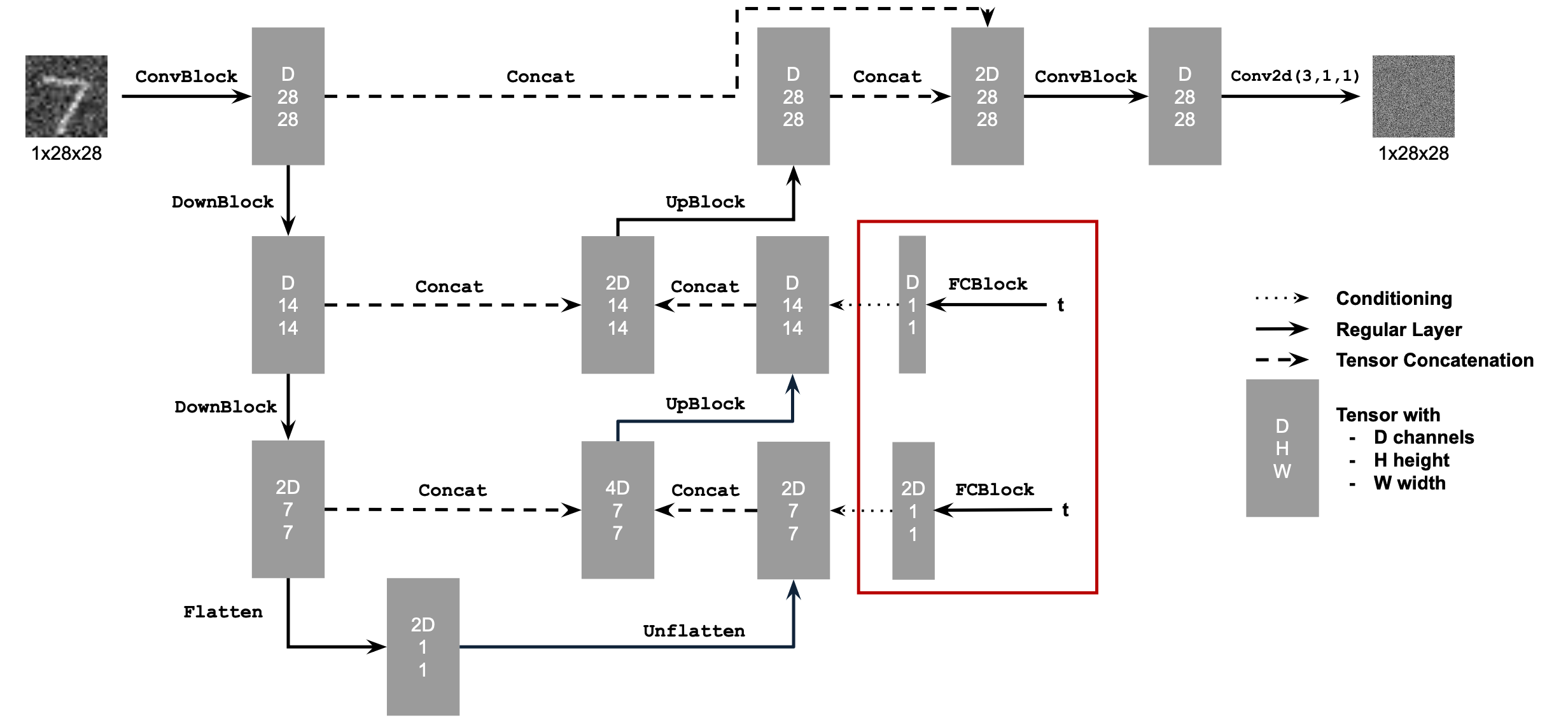
We have a new loss function, but we have a new variable timestep t. This means we need to inject this value into our UNet.
Part B - Section 2.1: Adding Time Conditioning to UNet
 Time Conditioning
|
We need to add FCBlock to the Unflatten and UpBlock where the FCBlock is defined as:
\[Linear(GELU(Linear(tensor)))\]
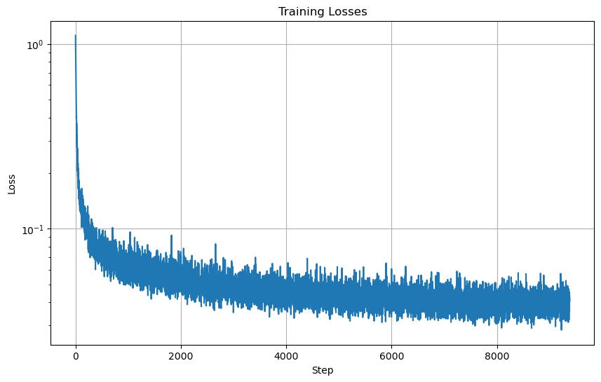
Part B - Section 2.2: Training the UNet
To train the model, we can load our optimizer, scheduler, and model again. We will use an Adam optimizer and an
exponential learning rate decay scheduler.
In the forward process, we randomly sample t and add noise to input image/tensor. We can sample the alpha bar value
from the scheduler. Then to get xt, we can calculate it with:
\[
x_t = \sqrt{\bar{\alpha}}x_0 + \sqrt{1 - \bar{\alpha}} * noise.
\]
Then we can get the predicted noise from the UNet using xt and run MSE Loss on the
predicted noise and the noised image/tensor we got earlier.
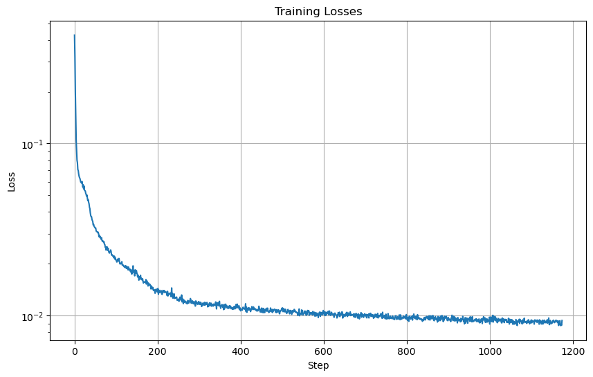
 Training Losses
|
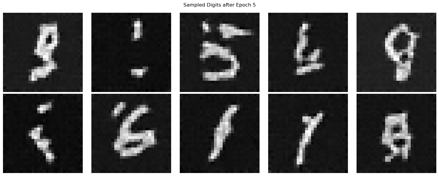
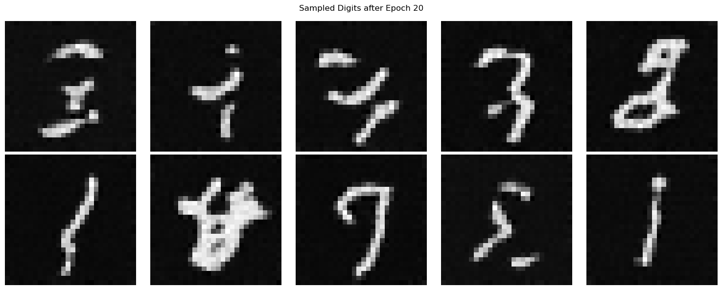
Part B - Section 2.3: Sampling from the UNet
To sample from our model, we first randomly sample a noised image. Then we iterate timesteps t through T = 300 steps, where at each step, we sample our
alpha values given t and then get a tensor z based on xt where if the timestep t is less than 1, the value is zero. We then get the
predicted noise from the UNet using xt and t. Each step, we find:
\[
(1 / \sqrt{{\alpha_t}}) * (x_t - (1 - \alpha_t) / \sqrt{1 - \bar\alpha_t} * noise) + \sqrt{1 - \alpha_t} * z
\]
 5 Epochs
|
 20 Epochs
|
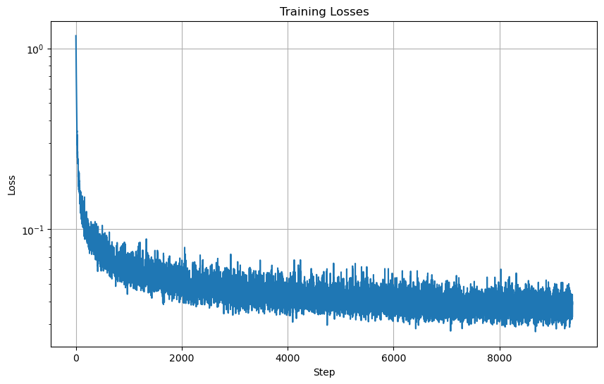
Part B - Section 2.4: Adding Class-Conditioning to UNet
Here, we will adding two more FCBlocks to our UNet. We have a class-conditioning vector c but we will make it a one-hot vector when
passing it into the FCBlock. We will add the new FCBlocks to the Unflatten and UpBlock.
 Training Losses
|
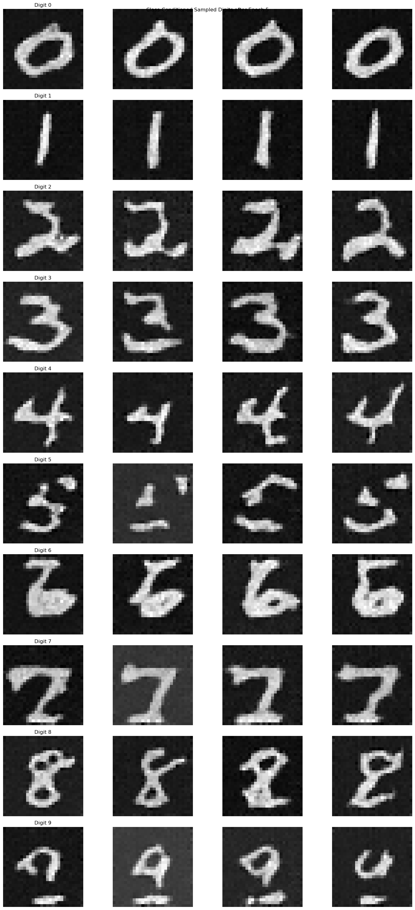
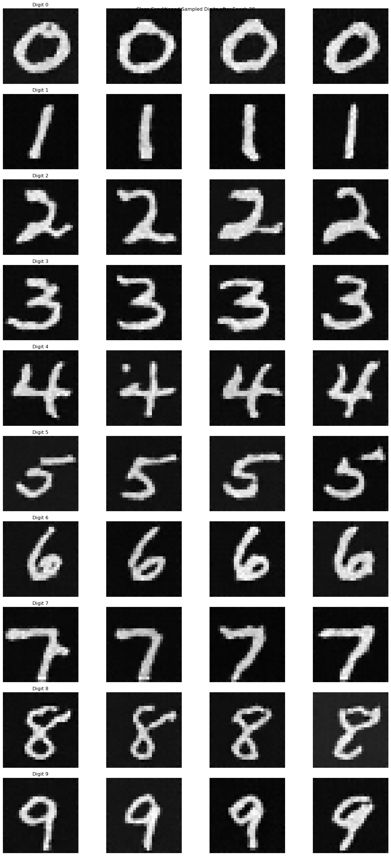
Part B - Section 2.5: Sampling from the Class-Conditioned UNet
For sampling, we will include classifer-free guidance, using a gamma value of 5.0.
\[
\epsilon = \epsilon_u + \gamma(\epsilon_c - \epsilon_u)
\]
where εu is the unconditioned predicted noise and εc is the conditioned predicted noise. Then each
step, we find like before:
\[
(1 / \sqrt{{\alpha_t}}) * (x_t - (1 - \alpha_t) / \sqrt{1 - \bar\alpha_t} * noise) + \sqrt{1 - \alpha_t} * z
\]
 5 Epochs
|
 20 Epochs
|
